
前回は,フーリエ変換を用いて2つの信号間の周波数空間での相関を評価するコヒーレンス,そして,相関のある周波数成分間の位相差を測るフェイズを紹介しました。
今回は,ウェーブレット変換を用いて,同様にウェーブレットコヒーレンスとウェーブレットフェイズを解析します。ウェーブレット変換を使用することによって,STFTが苦手とする過渡的な信号の解析により適した手法が得られます。
macOS Big Sur, python3.7.9
連続ウェーブレット変換 (復習)
復習になりますが,連続ウェーブレット変換を離散信号 $(x_i)_{i=0}^N = x_0, x_1, \dots, x_{N-1}$ に適用する場合,マザーウェーブレット $\psi$ を用意して
$$
W_n(s) = \sum_{n’=0}^{N-1} x_n\psi^*\left(\frac{(n’-n)\Delta t}{s}\right)
$$
とすれば良いことを述べました。
$W_n(s)$ は $n$ (時刻に対応するインデックス) におけるスケール $s$ のウェーブレット変換を意味します。
以後,離散信号 $(x_i)_{i=0}^N$ に関するウェーブレット変換を,右上にそれを明示して,$W_n^x(s)$ と表記します。
ウェーブレットコヒーレンスとフェイズ
STFTと同じように,2つの信号に対して,コヒーレンスとフェイズを定義することができます。
ウェーブレット(二乗)コヒーレンス (wavelet coherence)を
$$
\mathrm{coh}_n^2(s) = \frac{|\langle s^{-1} W_n^{xy}(s)\rangle|^2}{\langle s^{-1} |W_n^{x}(s)|^2\rangle\langle s^{-1} |W_n^{y}(s)|^2\rangle}
$$
と定義します。ここでも,周波数空間での平滑化が必要 (さもなければ,$\mathrm{coh}^2_n$ は恒等的に1になってしまいます) で,$\langle\cdot\rangle$ はスケールおよび時間領域で平滑化をしていることを示しています。
周波数平滑としては,Torrence & Compo (1998)の論文にあるものを使用することが多いようです。具体的には
$$
\langle W_n(s)\rangle = \mathcal{S}_{\mathrm{time}}(\mathcal{S}_{\mathrm{scale}}(W_n(s)))
$$
として,時間およびスケール( ≒ 周波数) の平滑化オペレータ $\mathcal{S}_{\mathrm{time}}$ と $\mathcal{S}_{\mathrm{scale}}$ に分けて,それぞれ
$$
\mathcal{S}_{\mathrm{time}}(W_n(s)) = W_n(s)\ast e^{t^2/(2s^2)} \\\mathcal{S}_{\mathrm{scale}}(W_n(s)) = W_n(s)\ast \Pi_s(\Delta j_0/\Delta j)
$$
とします。$\ast$ は畳み込み,$\Pi$ は引数で与えられた幅を持つ矩形関数です。畳み込みで表していますが,要するに移動平均をかけています。関数 $\Pi_s(\Delta j_0/\Delta j)$ の意味を理解するには,スケールの離散化を思い出す必要があります。スケール $s$ は,
$$
s_j = s_0\cdot 2^{j\Delta j}, \quad j = 0, 1, \dots, J \\J = \frac{1}{\Delta j}\log_2\left(\frac{N\Delta t}{s_0}\right)
$$
と離散化されていましたので,($s$ の空間で) 一様な幅の矩形関数で移動平均を取るわけには行きません。
関数 $\Pi_s(\Delta j_0/\Delta j)$ の意味は,($j$ の空間で) 幅 $\Delta j_0$ の矩形関数で平滑化することを意味します。
$\Delta j_0$ はウェーブレット関数の scale-decorrelation length [Torrence & Compo (1998)] で決めます。
$\omega_0 = 6$ のモルレーウェーブレットを使用するときは $\Delta j_0 = 0.6$ とします [Torrence & Compo (1998)],[Torrence & Webster (1999)]。
例えば,$\Delta j = 1/8$ の (周波数が 2 倍になる間に 8 刻みで離散化する) 場合,$\Delta j_0 = 0.6$ は周りの 4.8 個分の $j$ を巻き込んで平滑化することに対応します (したがって,$s$ が異なると,平滑化の幅 $\Delta s$ も異なります)。具体的な実装は,プログラムを参照してください。
ウェーブレットフェイズ (wavelet phase) は
$$
\theta_n(s) = \tan^{-1}\left(\frac{\mathrm{Im}(\langle s^{-1} W_n^{xy}(s)\rangle)}{\mathrm{Re}(\langle s^{-1} W_n^{xy}(s)\rangle)}\right)
$$
と定義します。これは
$$
\theta_{n}(s) = \text{($x(t)$に含まれるスケール$s$成分の位相)}-\text{($y(t)$に含まれるスケール$s$成分の位相)}
$$
という意味を持ちます。
ウェーブレットコヒーレンスとフェイズの実装
以上述べたことを基に,ウェーブレットコヒーレンスとウェーブレットフェイズの解析をpythonでコーディングしてみます。以下に実装例を示します。
import matplotlib as mpl
import matplotlib.pyplot as plt
import matplotlib.patheffects as path_effects
import numpy as np

#------------------------------------------------------------------------------
# 関数を定義
# 連続ウェーブレット変換を行う関数
def CWT_Morlet(tm, sig):
    dj = 0.125
    dt = tm[1] - tm[0]
    n_cwt = int(2**(np.ceil(np.log2(len(sig)))))

    # --- 後で使うパラメータを定義
    omega0 = 6.0
    s0 = 2.0*dt
    J = int(np.log2(n_cwt*dt/s0)/dj)

    # --- スケール
    s = s0*2.0**(dj*np.arange(0, J+1, 1))

    # --- n_cwt個のデータになるようにゼロパディングをして,DC成分を除く
    x = np.zeros(n_cwt)
    x[0:len(sig)] = sig[0:len(sig)] - np.mean(sig)

    # --- omega array
    omega = 2.0*np.pi*np.fft.fftfreq(n_cwt, dt)

    # --- FFTを使って離散ウェーブレット変換する
    X = np.fft.fft(x) # eq.(3)
    cwt = np.zeros((J+1, n_cwt), dtype=complex) # CWT array

    Hev = np.array(omega > 0.0)
    for j in range(J+1):
        Psi = np.sqrt(2.0*np.pi*s[j]/dt)*np.pi**(-0.25)*np.exp(-(s[j]*omega-omega0)**2/2.0)*Hev
        cwt[j, :] = np.fft.ifft(X*np.conjugate(Psi))

    s_to_f = (omega0 + np.sqrt(2 + omega0**2)) / (4.0*np.pi)
    freq_cwt = s_to_f / s
    cwt = cwt[:, 0:len(sig)]

    # --- cone of interference
    COI = np.zeros_like(tm)
    COI[0] = 0.5/dt
    COI[1:len(tm)//2] = np.sqrt(2)*s_to_f/tm[1:len(tm)//2]
    COI[len(tm)//2:-1] = np.sqrt(2)*s_to_f/(tm[-1]-tm[len(tm)//2:-1])
    COI[-1] = 0.5/dt

    return s, cwt, freq_cwt, COI

def smoothing(dt, s, W):
    dj = 0.125
    n_s, n_t = W.shape
    W_smthd = W

    # --- 時間方向の平滑化
    for j in range(n_s):
        W_temp = np.concatenate([np.zeros_like(W[j, :]), W[j, :],np.zeros_like(W[j, :])])
        tm_wndw = np.arange(-np.round(n_t), np.round(n_t))*dt
        krnl = np.exp(-(tm_wndw)**2/(2*s[j]**2))
        W_smthd[j, :] = (np.convolve(W_temp, krnl, mode='same')/np.sum(krnl))[n_t:2*n_t]

    # --- スケール方向の平滑化
    for i in range(n_t):
        dcrr = int(np.floor(0.6/(2*dj)))
        krnl = np.concatenate([[np.mod(dcrr, 1)], np.ones(dcrr), [np.mod(dcrr, 1)]])
        W_smthd[:, i] = np.convolve(W_smthd[:, i], krnl, mode='same')/np.sum(krnl)

    return W_smthd

#------------------------------------------------------------------------------
# テスト信号の生成
dt = 1.0e-4
tms = 0.0
tme = 2.0
tm01 = np.arange(tms, tme, dt)
tm02 = tm01

# np.random.seed(1234)
sig01 = np.random.randn(len(tm02))*0.05
sig01[tm01 < 0.3] += np.sin(2.0*np.pi*5.0e1*tm01[tm01 < 0.3])
sig01[(0.5 < tm01) & (tm01 < 0.8)] += np.sin(2.0*np.pi*1.0e2*tm01[(0.5 < tm01) & (tm01 < 0.8)])
sig01[(1.0 < tm01) & (tm01 < 1.3)] += np.sin(2.0*np.pi*1.5e2*tm01[(1.0 < tm01) & (tm01 < 1.3)])
sig01[(1.5 < tm01) & (tm01 < 1.8)] += np.sin(2.0*np.pi*2.0e2*tm01[(1.5 < tm01) & (tm01 < 1.8)])

sig02 = np.sin(2.0*np.pi*5.0e1*tm02) + 0.1*np.sin(2.0*np.pi*1.5e2*tm02 + np.pi/2.0) + np.random.randn(len(tm02))*0.05

#------------------------------------------------------------------------------
# 諸々の設定
freq_upper = 3.0e2 # 表示する周波数の上限

out_fig_path = "wcoh-wphase.png"

#------------------------------------------------------------------------------
# 連続ウェーブレット変換を実行
s01, cwt01, freq_cwt01, COI01 = CWT_Morlet(tm01, sig01)
s02, cwt02, freq_cwt02, COI02 = CWT_Morlet(tm02, sig02)

# クロススペクトル
xwt = cwt01*np.conjugate(cwt02)

# コヒーレンスとフェイズ
cwt01_pw_smthd = smoothing(dt, s01, np.abs(cwt01)**2*np.array([1.0/s01]).T)
cwt02_pw_smthd = smoothing(dt, s02, np.abs(cwt02)**2*np.array([1.0/s02]).T)
xwt_smthd = smoothing(dt, s01, xwt*np.array([1.0/s01]).T)

wcoh = np.abs(xwt_smthd)**2 / (cwt01_pw_smthd*cwt02_pw_smthd)
wphs = np.rad2deg(np.arctan2(np.imag(xwt_smthd), np.real(xwt_smthd)))


#------------------------------------------------------------------------------
# 結果のプロット
# 解析結果の可視化
figsize = (210/25.4, 294/25.4)
dpi = 200
fig = plt.figure(figsize=figsize, dpi=dpi)

# 図の設定 (全体)
plt.rcParams['xtick.direction'] = 'in'
plt.rcParams['xtick.top'] = True
plt.rcParams['xtick.major.size'] = 6
plt.rcParams['xtick.minor.size'] = 3
plt.rcParams['xtick.minor.visible'] = True
plt.rcParams['ytick.direction'] = 'in'
plt.rcParams['ytick.right'] = True
plt.rcParams['ytick.major.size'] = 6
plt.rcParams['ytick.minor.size'] = 3
plt.rcParams['ytick.minor.visible'] = True
plt.rcParams["font.size"] = 14
plt.rcParams['font.family'] = 'Helvetica'


# プロット枠の設定
ax01 = fig.add_axes([0.125, 0.79, 0.70, 0.08])
ax02 = fig.add_axes([0.125, 0.59, 0.70, 0.08])

ax_cwt01 = fig.add_axes([0.125, 0.68, 0.70, 0.10])
cb_cwt01 = fig.add_axes([0.85, 0.68, 0.02, 0.10])
ax_cwt02 = fig.add_axes([0.125, 0.48, 0.70, 0.10])
cb_cwt02 = fig.add_axes([0.85, 0.48, 0.02, 0.10])

ax_xwt = fig.add_axes([0.125, 0.33, 0.70, 0.10])
cb_xwt = fig.add_axes([0.85, 0.33, 0.02, 0.10])
ax_wcoh = fig.add_axes([0.125, 0.22, 0.70, 0.10])
cb_wcoh = fig.add_axes([0.85, 0.22, 0.02, 0.10])
ax_wphs = fig.add_axes([0.125, 0.10, 0.70, 0.10])
cb_wphs = fig.add_axes([0.85, 0.10, 0.02, 0.10])


# ---------------------------
# テスト信号 sig01 のプロット
ax01.set_xlim(tms, tme)
ax01.set_xlabel('')
ax01.tick_params(labelbottom=False)
ax01.set_ylabel('x (sig01)')

ax01.plot(tm01, sig01, c='black')

# ---------------------------
# テスト信号 sig02 のプロット
ax02.set_xlim(tms, tme)
ax02.set_xlabel('')
ax02.tick_params(labelbottom=False)
ax02.set_ylabel('y (sig02)')

ax02.plot(tm02, sig02, c='black')

# ---------------------------
# テスト信号 sig01 のスカログラムのプロット
ax_cwt01.set_xlim(tms, tme)
ax_cwt01.set_xlabel('')
ax_cwt01.tick_params(labelbottom=False)
ax_cwt01.set_ylim(0, freq_upper)
ax_cwt01.set_ylabel('frequency\n(Hz)')

norm = mpl.colors.Normalize(vmin=np.log10(np.abs(cwt01[freq_cwt01 < freq_upper, :])**2).min(),
                            vmax=np.log10(np.abs(cwt01[freq_cwt01 < freq_upper, :])**2).max())
cmap = mpl.cm.jet

ax_cwt01.contourf(tm01, freq_cwt01, np.log10(np.abs(cwt01)**2),
                 norm=norm, levels=256, cmap=cmap)

# Cone of Interference のプロット
ax_cwt01.fill_between(tm01, COI01, fc='w', hatch='x', alpha=0.5)
ax_cwt01.plot(tm01, COI01, '--', color='black')

ax_cwt01.text(0.99, 0.97, "spectrogram", color='white', ha='right', va='top',
              path_effects=[path_effects.Stroke(linewidth=2, foreground='black'),
                            path_effects.Normal()],
              transform=ax_cwt01.transAxes)

mpl.colorbar.ColorbarBase(cb_cwt01, cmap=cmap, norm=norm,
                          orientation="vertical",
                          label='$\log_{10}|W^x|^2$')

# ---------------------------
# テスト信号 sig02 のスカログラムのプロット
ax_cwt02.set_xlim(tms, tme)
ax_cwt02.set_xlabel('')
ax_cwt02.tick_params(labelbottom=True)
ax_cwt02.set_ylim(0, freq_upper)
ax_cwt02.set_ylabel('frequency\n(Hz)')


norm = mpl.colors.Normalize(vmin=np.log10(np.abs(cwt02[freq_cwt02 < freq_upper, :])**2).min(),
                            vmax=np.log10(np.abs(cwt02[freq_cwt02 < freq_upper, :])**2).max())
ax_cwt02.contourf(tm02, freq_cwt02, np.log10(np.abs(cwt02)**2),
                 norm=norm, levels=256, cmap=cmap)

ax_cwt02.text(0.99, 0.97, "spectrogram", color='white', ha='right', va='top',
              path_effects=[path_effects.Stroke(linewidth=2, foreground='black'),
                            path_effects.Normal()],
              transform=ax_cwt02.transAxes)

# Cone of Interference のプロット
ax_cwt02.fill_between(tm02, COI02, fc='w', hatch='x', alpha=0.5)
ax_cwt02.plot(tm02, COI02, '--', color='black')

mpl.colorbar.ColorbarBase(cb_cwt02, cmap=cmap, norm=norm,
                          orientation="vertical",
                          label='$\log_{10}|W^y|^2$')

# ---------------------------
# テスト信号 sig01 と sig02 のクロスウェーブレットのプロット
ax_xwt.set_xlim(tms, tme)
ax_xwt.set_xlabel('')
ax_xwt.tick_params(labelbottom=False)
ax_xwt.set_ylim(0, freq_upper)
ax_xwt.set_ylabel('frequency\n(Hz)')


norm = mpl.colors.Normalize(vmin=np.log10(np.abs(xwt[freq_cwt01 < freq_upper, :])).min(),
                            vmax=np.log10(np.abs(xwt[freq_cwt01 < freq_upper, :])).max())

ax_xwt.contourf(tm01, freq_cwt01, np.log10(np.abs(xwt)),
                norm=norm, levels=256, cmap=cmap)

ax_xwt.text(0.99, 0.97, "cross-spectrum", color='white', ha='right', va='top',
            path_effects=[path_effects.Stroke(linewidth=2, foreground='black'),
                          path_effects.Normal()],
            transform=ax_xwt.transAxes)

# Cone of Interference のプロット
ax_xwt.fill_between(tm01, COI01, fc='w', hatch='x', alpha=0.5)
ax_xwt.plot(tm01, COI01, '--', color='black')

mpl.colorbar.ColorbarBase(cb_xwt, cmap=cmap, norm=norm,
                          orientation="vertical",
                          label='$\log_{10}|W^xW^{y*}|$')

# ---------------------------
# テスト信号 sig01 と sig02 のウェーブレットコヒーレンスのプロット
ax_wcoh.set_xlim(tms, tme)
ax_wcoh.set_xlabel('')
ax_wcoh.tick_params(labelbottom=False)
ax_wcoh.set_ylim(0, freq_upper)
ax_wcoh.set_ylabel('frequency\n(Hz)')

norm = mpl.colors.Normalize(vmin=0.0, vmax=1.0)
ax_wcoh.contourf(tm01, freq_cwt01, wcoh,
                 norm=norm, levels=10, cmap=cmap)

ax_wcoh.text(0.99, 0.97, "coherence", color='white', ha='right', va='top',
             path_effects=[path_effects.Stroke(linewidth=2, foreground='black'),
                           path_effects.Normal()],
             transform=ax_wcoh.transAxes)

# Cone of Interference のプロット
ax_wcoh.fill_between(tm01, COI01, fc='w', hatch='x', alpha=0.5)
ax_wcoh.plot(tm01, COI01, '--', color='black')

mpl.colorbar.ColorbarBase(cb_wcoh, cmap=cmap, norm=norm,
                          boundaries=np.linspace(0, 1, 11),
                          orientation="vertical",
                          label='coherence')

# ---------------------------
# テスト信号 sig01 と sig02 のウェーブレットフェイズのプロット
ax_wphs.set_xlim(tms, tme)
ax_wphs.set_xlabel('time (s)')
ax_wphs.tick_params(labelbottom=True)
ax_wphs.set_ylim(0, freq_upper)
ax_wphs.set_ylabel('frequency\n(Hz)')

norm = mpl.colors.Normalize(vmin=-180.0, vmax=180.0)
cmap = mpl.cm.hsv
ax_wphs.contourf(tm01, freq_cwt01, np.where(wcoh >= 0.75, wphs, None),
                 norm=norm, levels=16, cmap=cmap)

ax_wphs.text(0.99, 0.97, "phase", color='white', ha='right', va='top',
             path_effects=[path_effects.Stroke(linewidth=2, foreground='black'),
                           path_effects.Normal()],
             transform=ax_wphs.transAxes)

# Cone of Interference のプロット
ax_wphs.fill_between(tm01, COI01, fc='w', hatch='x', alpha=0.5)
ax_wphs.plot(tm01, COI01, '--', color='black')

mpl.colorbar.ColorbarBase(cb_wphs, cmap=cmap,
                          norm=norm,
                          boundaries=np.linspace(-180.0, 180.0, 17),
                          orientation="vertical",
                          label='phase (deg)')

#-----------------------------------------------------------------------------
# 図の出力
plt.savefig(out_fig_path, transparent=False)
プログラムを実行する
上で記述したコードは wcoh-wphase-demo.pyという名前のファイルとして,好きなディレクトリ(ここでは~/Desktop/LabCode/python/wcoh-wphaseとします)に保存します。
ターミナルを開き,
$ cd Desktop/LabCode/python/wcoh-wphaseと入力し,ディレクトリを移動します。あとは以下のコマンドで coh-phase-demo.pyを実行するだけです。( $マークは無視してください)。
$ python3 wcoh-wphase-demo.py実行結果
~/Desktop/LabCode/python/coh-phase にwcoh-wphase.pngというファイルができて,以下のようになっていれば成功です!(実行にやや時間がかかります)
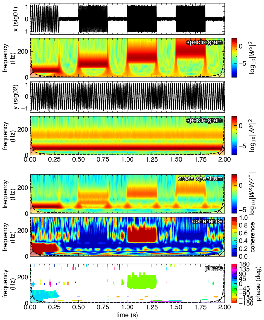
一段目から四段目はテスト信号とそのスカログラムです。
テスト信号として,
$$
\mathrm{sig01}(t) = \mathcal{N}_{\mu=0, \sigma=0.05}(t) + \begin{cases}\sin(2\pi\times 50\times t), & 0\ \mathrm{s}\le t < 0.3\ \mathrm{s}, \\\sin(2\pi\times 100\times t), & 0.5\ \mathrm{s} <t < 0.8\ \mathrm{s}, \\\sin(2\pi\times 150\times t), & 1.0\ \mathrm{s} < t < 1.3\ \mathrm{s}, \\\sin(2\pi\times 200\times t), &1.5 \ \mathrm{s}< t < 1.8\ \mathrm{s}, \end{cases},
$$
$$
\mathrm{sig02}(t) = \mathcal{N}_{\mu=0, \sigma=0.05}(t) + \sin(2\pi\times 50\times t) +0.1\sin(2\pi\times 150\times t + \pi/2)
$$
が用いられています。ここで,$\mathcal{N}_{\mu=0, \sigma=0.05}(t)$ は平均0,標準偏差0.05のガウシアンノイズを表します。sig02に含まれる150 kHzの成分はsig01よりも90度 (=π/2 ラジアン) 進んだものを入れています(たとえば,$\sin(x)$ と$\sin(x+\pi/2) = \cos(x)$ のグラフを考えてください。
五段目はウェーブレットクロススカログラムを示しています。
六段目はウェーブレットコヒーレンス,七段目はウェーブレットフェイズです。ウェーブレットコヒーレンスは2つの信号に含まれる周波数成分が一致するとき,つまり,0 s ~ 0.3 sと1.0 s~ 1.3 sにおいて,それぞれ,50 Hz付近と150 kHz付近で,1に近くなっていることがわかります。
また,その時のウェーブレットフェイズ(位相差)はそれぞれ,0度(sig01に含まれる50 kHzの成分とsig02に含まれる50 kHzの成分の位相の間にずれはない)と–90度(sig01に含まれる150 kHzの成分は,sig02に含まれる150 kHzの成分よりも位相が90度遅れている)となっており,テスト信号から想定される結果通りとなっています。
コードの解説
コードの解説をしていきます。
import matplotlib as mpl
import matplotlib.pyplot as plt
import matplotlib.patheffects as path_effects
import numpy as np
必要なモジュールをインポートします。
#------------------------------------------------------------------------------
# 関数を定義
# 連続ウェーブレット変換を行う関数
def CWT_Morlet(tm, sig):
    dj = 0.125
    dt = tm[1] - tm[0]
    n_cwt = int(2**(np.ceil(np.log2(len(sig)))))

    # --- 後で使うパラメータを定義
    omega0 = 6.0
    s0 = 2.0*dt
    J = int(np.log2(n_cwt*dt/s0)/dj)

    # --- スケール
    s = s0*2.0**(dj*np.arange(0, J+1, 1))

    # --- n_cwt個のデータになるようにゼロパディングをして,DC成分を除く
    x = np.zeros(n_cwt)
    x[0:len(sig)] = sig[0:len(sig)] - np.mean(sig)

    # --- omega array
    omega = 2.0*np.pi*np.fft.fftfreq(n_cwt, dt)

    # --- FFTを使って離散ウェーブレット変換する
    X = np.fft.fft(x) # eq.(3)
    cwt = np.zeros((J+1, n_cwt), dtype=complex) # CWT array

    Hev = np.array(omega > 0.0)
    for j in range(J+1):
        Psi = np.sqrt(2.0*np.pi*s[j]/dt)*np.pi**(-0.25)*np.exp(-(s[j]*omega-omega0)**2/2.0)*Hev
        cwt[j, :] = np.fft.ifft(X*np.conjugate(Psi))

    s_to_f = (omega0 + np.sqrt(2 + omega0**2)) / (4.0*np.pi)
    freq_cwt = s_to_f / s
    cwt = cwt[:, 0:len(sig)]

    # --- cone of interference
    COI = np.zeros_like(tm)
    COI[0] = 0.5/dt
    COI[1:len(tm)//2] = np.sqrt(2)*s_to_f/tm[1:len(tm)//2]
    COI[len(tm)//2:-1] = np.sqrt(2)*s_to_f/(tm[-1]-tm[len(tm)//2:-1])
    COI[-1] = 0.5/dt

    return s, cwt, freq_cwt, COI

def smoothing(dt, s, W):
    dj = 0.125
    n_s, n_t = W.shape
    W_smthd = W

    # --- 時間方向の平滑化
    for j in range(n_s):
        W_temp = np.concatenate([np.zeros_like(W[j, :]), W[j, :],np.zeros_like(W[j, :])])
        tm_wndw = np.arange(-np.round(n_t), np.round(n_t))*dt
        krnl = np.exp(-(tm_wndw)**2/(2*s[j]**2))
        W_smthd[j, :] = (np.convolve(W_temp, krnl, mode='same')/np.sum(krnl))[n_t:2*n_t]

    # --- スケール方向の平滑化
    for i in range(n_t):
        dcrr = int(np.floor(0.6/(2*dj)))
        krnl = np.concatenate([[np.mod(dcrr, 1)], np.ones(dcrr), [np.mod(dcrr, 1)]])
        W_smthd[:, i] = np.convolve(W_smthd[:, i], krnl, mode='same')/np.sum(krnl)

    return W_smthd
繰り返し使用するウェーブレット変換と,スカログラムの時間およびスケール方向の平滑化を関数として定義しておきます。
#------------------------------------------------------------------------------
# テスト信号の生成
dt = 1.0e-4
tms = 0.0
tme = 2.0
tm01 = np.arange(tms, tme, dt)
tm02 = tm01

# np.random.seed(1234)
sig01 = np.random.randn(len(tm02))*0.05
sig01[tm01 < 0.3] += np.sin(2.0*np.pi*5.0e1*tm01[tm01 < 0.3])
sig01[(0.5 < tm01) & (tm01 < 0.8)] += np.sin(2.0*np.pi*1.0e2*tm01[(0.5 < tm01) & (tm01 < 0.8)])
sig01[(1.0 < tm01) & (tm01 < 1.3)] += np.sin(2.0*np.pi*1.5e2*tm01[(1.0 < tm01) & (tm01 < 1.3)])
sig01[(1.5 < tm01) & (tm01 < 1.8)] += np.sin(2.0*np.pi*2.0e2*tm01[(1.5 < tm01) & (tm01 < 1.8)])

sig02 = np.sin(2.0*np.pi*5.0e1*tm02) + 0.1*np.sin(2.0*np.pi*1.5e2*tm02 + np.pi/2.0) + np.random.randn(len(tm02))*0.05
テスト信号を生成します。上で述べたように,テスト信号として
$$
\mathrm{sig01}(t) = \mathcal{N}_{\mu=0, \sigma=0.05}(t) + \begin{cases}\sin(2\pi\times 50\times t), & 0\ \mathrm{s}\le t < 0.3\ \mathrm{s}, \\\sin(2\pi\times 100\times t), & 0.5\ \mathrm{s} <t < 0.8\ \mathrm{s}, \\\sin(2\pi\times 150\times t), & 1.0\ \mathrm{s} < t < 1.3\ \mathrm{s}, \\\sin(2\pi\times 200\times t), &1.5 \ \mathrm{s}< t < 1.8\ \mathrm{s}, \end{cases},
$$
$$
\\\mathrm{sig02}(t) = \mathcal{N}_{\mu=0, \sigma=0.05}(t) + \sin(2\pi\times 50\times t) +0.1\sin(2\pi\times 150\times t + \pi/2)
$$
を用いました。
#------------------------------------------------------------------------------
# 諸々の設定
freq_upper = 3.0e2 # 表示する周波数の上限

out_fig_path = "wcoh-wphase.png"
この部分はスカログラムの上限の周波数と出力される図のファイル名の設定です。
#------------------------------------------------------------------------------
# 連続ウェーブレット変換を実行
s01, cwt01, freq_cwt01, COI01 = CWT_Morlet(tm01, sig01)
s02, cwt02, freq_cwt02, COI02 = CWT_Morlet(tm02, sig02)

# クロススペクトル
xwt = cwt01*np.conjugate(cwt02)

# コヒーレンスとフェイズ
cwt01_pw_smthd = smoothing(dt, s01, np.abs(cwt01)**2*np.array([1.0/s01]).T)
cwt02_pw_smthd = smoothing(dt, s02, np.abs(cwt02)**2*np.array([1.0/s02]).T)
xwt_smthd = smoothing(dt, s01, xwt*np.array([1.0/s01]).T)

wcoh = np.abs(xwt_smthd)**2 / (cwt01_pw_smthd*cwt02_pw_smthd)
wphs = np.rad2deg(np.arctan2(np.imag(xwt_smthd), np.real(xwt_smthd)))
上で述べた定義に従って,ウェーブレットクロススペクトル,ウェーブレットコヒーレンスとウェーブレットフェイズを計算します。
#------------------------------------------------------------------------------
# 結果のプロット
# 解析結果の可視化
figsize = (210/25.4, 294/25.4)
dpi = 200
fig = plt.figure(figsize=figsize, dpi=dpi)

# 図の設定 (全体)
plt.rcParams['xtick.direction'] = 'in'
plt.rcParams['xtick.top'] = True
plt.rcParams['xtick.major.size'] = 6
plt.rcParams['xtick.minor.size'] = 3
plt.rcParams['xtick.minor.visible'] = True
plt.rcParams['ytick.direction'] = 'in'
plt.rcParams['ytick.right'] = True
plt.rcParams['ytick.major.size'] = 6
plt.rcParams['ytick.minor.size'] = 3
plt.rcParams['ytick.minor.visible'] = True
plt.rcParams["font.size"] = 14
plt.rcParams['font.family'] = 'Helvetica'


# プロット枠の設定
ax01 = fig.add_axes([0.125, 0.79, 0.70, 0.08])
ax02 = fig.add_axes([0.125, 0.59, 0.70, 0.08])

ax_cwt01 = fig.add_axes([0.125, 0.68, 0.70, 0.10])
cb_cwt01 = fig.add_axes([0.85, 0.68, 0.02, 0.10])
ax_cwt02 = fig.add_axes([0.125, 0.48, 0.70, 0.10])
cb_cwt02 = fig.add_axes([0.85, 0.48, 0.02, 0.10])

ax_xwt = fig.add_axes([0.125, 0.33, 0.70, 0.10])
cb_xwt = fig.add_axes([0.85, 0.33, 0.02, 0.10])
ax_wcoh = fig.add_axes([0.125, 0.22, 0.70, 0.10])
cb_wcoh = fig.add_axes([0.85, 0.22, 0.02, 0.10])
ax_wphs = fig.add_axes([0.125, 0.10, 0.70, 0.10])
cb_wphs = fig.add_axes([0.85, 0.10, 0.02, 0.10])


# ---------------------------
# テスト信号 sig01 のプロット
ax01.set_xlim(tms, tme)
ax01.set_xlabel('')
ax01.tick_params(labelbottom=False)
ax01.set_ylabel('x (sig01)')

ax01.plot(tm01, sig01, c='black')

# ---------------------------
# テスト信号 sig02 のプロット
ax02.set_xlim(tms, tme)
ax02.set_xlabel('')
ax02.tick_params(labelbottom=False)
ax02.set_ylabel('y (sig02)')

ax02.plot(tm02, sig02, c='black')

# ---------------------------
# テスト信号 sig01 のスカログラムのプロット
ax_cwt01.set_xlim(tms, tme)
ax_cwt01.set_xlabel('')
ax_cwt01.tick_params(labelbottom=False)
ax_cwt01.set_ylim(0, freq_upper)
ax_cwt01.set_ylabel('frequency\n(Hz)')

norm = mpl.colors.Normalize(vmin=np.log10(np.abs(cwt01[freq_cwt01 < freq_upper, :])**2).min(),
                            vmax=np.log10(np.abs(cwt01[freq_cwt01 < freq_upper, :])**2).max())
cmap = mpl.cm.jet

ax_cwt01.contourf(tm01, freq_cwt01, np.log10(np.abs(cwt01)**2),
                 norm=norm, levels=256, cmap=cmap)

# Cone of Interference のプロット
ax_cwt01.fill_between(tm01, COI01, fc='w', hatch='x', alpha=0.5)
ax_cwt01.plot(tm01, COI01, '--', color='black')

ax_cwt01.text(0.99, 0.97, "spectrogram", color='white', ha='right', va='top',
              path_effects=[path_effects.Stroke(linewidth=2, foreground='black'),
                            path_effects.Normal()],
              transform=ax_cwt01.transAxes)

mpl.colorbar.ColorbarBase(cb_cwt01, cmap=cmap, norm=norm,
                          orientation="vertical",
                          label='$\log_{10}|W^x|^2$')

# ---------------------------
# テスト信号 sig02 のスカログラムのプロット
ax_cwt02.set_xlim(tms, tme)
ax_cwt02.set_xlabel('')
ax_cwt02.tick_params(labelbottom=True)
ax_cwt02.set_ylim(0, freq_upper)
ax_cwt02.set_ylabel('frequency\n(Hz)')


norm = mpl.colors.Normalize(vmin=np.log10(np.abs(cwt02[freq_cwt02 < freq_upper, :])**2).min(),
                            vmax=np.log10(np.abs(cwt02[freq_cwt02 < freq_upper, :])**2).max())
ax_cwt02.contourf(tm02, freq_cwt02, np.log10(np.abs(cwt02)**2),
                 norm=norm, levels=256, cmap=cmap)

ax_cwt02.text(0.99, 0.97, "spectrogram", color='white', ha='right', va='top',
              path_effects=[path_effects.Stroke(linewidth=2, foreground='black'),
                            path_effects.Normal()],
              transform=ax_cwt02.transAxes)

# Cone of Interference のプロット
ax_cwt02.fill_between(tm02, COI02, fc='w', hatch='x', alpha=0.5)
ax_cwt02.plot(tm02, COI02, '--', color='black')

mpl.colorbar.ColorbarBase(cb_cwt02, cmap=cmap, norm=norm,
                          orientation="vertical",
                          label='$\log_{10}|W^y|^2$')

# ---------------------------
# テスト信号 sig01 と sig02 のクロスウェーブレットのプロット
ax_xwt.set_xlim(tms, tme)
ax_xwt.set_xlabel('')
ax_xwt.tick_params(labelbottom=False)
ax_xwt.set_ylim(0, freq_upper)
ax_xwt.set_ylabel('frequency\n(Hz)')


norm = mpl.colors.Normalize(vmin=np.log10(np.abs(xwt[freq_cwt01 < freq_upper, :])).min(),
                            vmax=np.log10(np.abs(xwt[freq_cwt01 < freq_upper, :])).max())

ax_xwt.contourf(tm01, freq_cwt01, np.log10(np.abs(xwt)),
                norm=norm, levels=256, cmap=cmap)

ax_xwt.text(0.99, 0.97, "cross-spectrum", color='white', ha='right', va='top',
            path_effects=[path_effects.Stroke(linewidth=2, foreground='black'),
                          path_effects.Normal()],
            transform=ax_xwt.transAxes)

# Cone of Interference のプロット
ax_xwt.fill_between(tm01, COI01, fc='w', hatch='x', alpha=0.5)
ax_xwt.plot(tm01, COI01, '--', color='black')

mpl.colorbar.ColorbarBase(cb_xwt, cmap=cmap, norm=norm,
                          orientation="vertical",
                          label='$\log_{10}|W^xW^{y*}|$')

# ---------------------------
# テスト信号 sig01 と sig02 のウェーブレットコヒーレンスのプロット
ax_wcoh.set_xlim(tms, tme)
ax_wcoh.set_xlabel('')
ax_wcoh.tick_params(labelbottom=False)
ax_wcoh.set_ylim(0, freq_upper)
ax_wcoh.set_ylabel('frequency\n(Hz)')

norm = mpl.colors.Normalize(vmin=0.0, vmax=1.0)
ax_wcoh.contourf(tm01, freq_cwt01, wcoh,
                 norm=norm, levels=10, cmap=cmap)

ax_wcoh.text(0.99, 0.97, "coherence", color='white', ha='right', va='top',
             path_effects=[path_effects.Stroke(linewidth=2, foreground='black'),
                           path_effects.Normal()],
             transform=ax_wcoh.transAxes)

# Cone of Interference のプロット
ax_wcoh.fill_between(tm01, COI01, fc='w', hatch='x', alpha=0.5)
ax_wcoh.plot(tm01, COI01, '--', color='black')

mpl.colorbar.ColorbarBase(cb_wcoh, cmap=cmap, norm=norm,
                          boundaries=np.linspace(0, 1, 11),
                          orientation="vertical",
                          label='coherence')

# ---------------------------
# テスト信号 sig01 と sig02 のウェーブレットフェイズのプロット
ax_wphs.set_xlim(tms, tme)
ax_wphs.set_xlabel('time (s)')
ax_wphs.tick_params(labelbottom=True)
ax_wphs.set_ylim(0, freq_upper)
ax_wphs.set_ylabel('frequency\n(Hz)')

norm = mpl.colors.Normalize(vmin=-180.0, vmax=180.0)
cmap = mpl.cm.hsv
ax_wphs.contourf(tm01, freq_cwt01, np.where(wcoh >= 0.75, wphs, None),
                 norm=norm, levels=16, cmap=cmap)

ax_wphs.text(0.99, 0.97, "phase", color='white', ha='right', va='top',
             path_effects=[path_effects.Stroke(linewidth=2, foreground='black'),
                           path_effects.Normal()],
             transform=ax_wphs.transAxes)

# Cone of Interference のプロット
ax_wphs.fill_between(tm01, COI01, fc='w', hatch='x', alpha=0.5)
ax_wphs.plot(tm01, COI01, '--', color='black')

mpl.colorbar.ColorbarBase(cb_wphs, cmap=cmap,
                          norm=norm,
                          boundaries=np.linspace(-180.0, 180.0, 17),
                          orientation="vertical",
                          label='phase (deg)')

#-----------------------------------------------------------------------------
# 図の出力
plt.savefig(out_fig_path, transparent=False)解析の結果をプロットします。前半の4つのプロット部分は前回の記事で詳しく説明したものと同じです。
後半3つ(クロススペクトル,コヒーレンス,フェイズ)に関してもほとんど同じですが,contourfのlevelsオプションでlevels=10やlevels=17として,わざと離散的に表現しています。
また,フェイズのカラーマップはhsvとし,–180度と180度が滑らかにつながるようにしています。フェイズはコヒーレンスが1に近い周波数でのみ意味を持ちますので,コヒーレンスが0.75以上の場合にのみ表示するようにしています。
参考文献
- C. Torrence and G. P. Compo, “A Practical Guide to Wavelet Analysis”, Bull. Amer. Meteor. Soc. 79, 61 (1998): https://journals.ametsoc.org/view/journals/bams/79/1/1520-0477_1998_079_0061_apgtwa_2_0_co_2.xml
- C. Torrence and P. J. Webster, “Interdecadal Changes in the ENSO–Monsoon System ”, J. Climate 12, 2679 (1999)