【Python】How to install Cartopy to handle geospatial data 【Cartopy】

Have you ever wanted to handle geospatial data (geography information system data, GIS data, or geospatial data) (data about a value on the earth where the position is expressed in latitude and longitude) in Python? For example, meteorological data (AMeDAS data for each location, grid point data (GPV data) on the numerical model output by numerical forecasting) is one of the typical types of GIS data.

Another article in the blog also introduces how to plot GIS data using a library called folium. This time, we will introduce Cartopy, a package for handling GIS data, and its basic usage.

Cartopy allows you to easily plot GIS data, for example, in different projections (Mercator, Conformal Azimuth, Lambert Conformal Conic…).

Tested Environment

macOS BigSur (11.7.1), python3.9.15, Cartopy0.21.0

What is Cartopy?

Cartopy is a package for handling GIS data with Python. Its development originally began at the UK Met Office.

Since the Earth is a sphere (or, more precisely, an ellipsoid), the Cartesian coordinate system we usually use is only locally satisfied.

Various projections are used to represent data on the Earth in two dimensions, and the data must be transformed appropriately. (Remember, for example, that the Mercator projection stretches the continents in the polar regions).

Cartopy does the tiresome stuff for your GIS data. Now, let’s install it!

How to Install Cartopy

Cartopy can be installed using pip or conda. This time, we will explain how to use homebrew and pip, which are the methods explained on the official website.

Before installing Cartopy itself, you need to install GEOS, Shapely, and pyshp, which Cartopy depends on (which it calls internally). The dependencies and links between these can be confusing, so they must be done in the order they are presented.

Anyway, first of all, let’s update homebrew ($the mark is a “prompt”. You don’t need to type it).

$ brew update

It may take some time if you have not updated for a while. Once the update is complete, install GEOS.

$ brew install geos

Once the installation is completed, install pyshp using pip.

$ pip3 install --upgrade pyshp

Next, Shapely requires building from source code. This requires to link with the GEOS installed above. Therefore, if you have already installed Shapely, you will need to uninstall it.

By tying pip3 list, you can check whether it is installed or not by looking at the list of installed packages that appear. If it is installed, typepip3 uninstall shapely(run the commented-out command to uninstall it.).

$ pip3 list
$ #pip3 uninstall shapely
$ pip3 install "shapely<2" --no-binary shapely

Install pkg-config, which is required when building Cartopy. After installation, PKG_CONFIG_PATHconfigure the settings.

$ brew install pkg-config
$ export PKG_CONFIG_PATH=/usr/local/bin/pkgconfig

If you complete the above, you are ready to install Cartopy with pip.

$ pip3 install cartopy

The installation is now complete!
If you install using the above method, currently (2022/11/30) Cartopy0.21.0 will be installed.

Plot a Map Around Japan

Program to Plot in Equirectangular Projection

Plot a map around Japan using the program on the gallery on the official website.

As a reference, we will show you the program to mark the location where Tsutenkaku (a landmark tower of Osaka) is located!

Write the code below and save it as a file name map-japan.py in the directory where you want to save the program and generated diagrams ( say ~/Desktop/LabCode/python/weather).

import cartopy.crs as ccrs
import cartopy.feature as cfeature
import matplotlib.pyplot as plt

fig = plt.figure(figsize=(294/25.4, 210/25.4))
ax = fig.add_axes([0.10, 0.10, 0.80, 0.80], projection=ccrs.PlateCarree())
# ---
# if you want to draw a map in another projection
# please uncomment out
# ax = fig.add_axes([0.10, 0.10, 0.80, 0.80], projection=ccrs.Mercator())
# ax = fig.add_axes([0.10, 0.10, 0.80, 0.80], projection=ccrs.Robinson())
# ax = fig.add_axes([0.10, 0.10, 0.80, 0.80], projection=ccrs.LambertCylindrical())
# ax = fig.add_axes([0.10, 0.10, 0.80, 0.80], projection=ccrs.LambertConformal())

ax.set_extent([120, 160, 20, 50], crs=ccrs.PlateCarree())
ax.add_feature(cfeature.LAND)
ax.add_feature(cfeature.OCEAN)
ax.add_feature(cfeature.COASTLINE)
ax.add_feature(cfeature.BORDERS, linestyle=':')
ax.add_feature(cfeature.LAKES)
ax.add_feature(cfeature.RIVERS)

# --- location of Tsutenkaku
ax.scatter(135+30/60+22.77/60/60, 34.0+39/60+9.13/60/60, transform=ccrs.PlateCarree())

# --- grids 
ax.gridlines(linestyle='dashed', color='gray', linewidth=0.5,  draw_labels=True)

plt.savefig('map-japan.png')

Executing the Program

Open a terminal window and enter:

$ cd Desktop/LabCode/python/weather/

to change the current working directory. Then, execute the program by

$ python3 map-japan.py

Execution Results

When you run it, you can find an image file named map-japan.png in ~/Desktop/LabCode/python/weather.

The execution is successful if you get the image below.

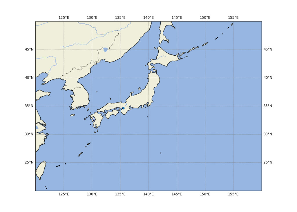
The first time you use Cartopy to plot a map (as well as the first time you use a map at that resolution), a download occurs, which may take some time. Also, a warning will appear on the terminal, but there is no need to worry.

You can also see that a blue dot is plotted at the location of Tsutenkaku, too!

Explanation of the Code

We will explain the source code written above

import cartopy.crs as ccrs
import cartopy.feature as cfeature
import matplotlib.pyplot as plt

First, import the necessary modules.

fig = plt.figure(figsize=(294/25.4, 210/25.4))
ax = fig.add_axes([0.10, 0.10, 0.80, 0.80], projection=ccrs.PlateCarree())
# ---
# if you want to draw a map in another projection
# please uncomment out
# ax = fig.add_axes([0.10, 0.10, 0.80, 0.80], projection=ccrs.Mercator())
# ax = fig.add_axes([0.10, 0.10, 0.80, 0.80], projection=ccrs.Robinson())
# ax = fig.add_axes([0.10, 0.10, 0.80, 0.80], projection=ccrs.LambertCylindrical())
# ax = fig.add_axes([0.10, 0.10, 0.80, 0.80], projection=ccrs.LambertConformal())

Configure the plot area. Here, we choose A4 landscape layout.

For the plot area, specify 10% from the left and 10% from the bottom of the paper as the lower left corner of the plot frame, and specify the plot frame size as 80% horizontally and 80% vertically of the paper.

Since we will be using the equirectangular projection, projection=ccrs.PlateCarree()we will add this to the options.

If you want to draw in a different projection method, change the argument of projection. For example, you can use a commented-out version. However, what is written here is just an example. There are many others available.

Also, as shown at the bottom, it is possible to input arguments like ccrs.LambertConformal(central_longitude=140), but if you use the default values, the expected chart may not appear.

ax.set_extent([120, 160, 20, 50], crs=ccrs.PlateCarree())
ax.add_feature(cfeature.LAND)
ax.add_feature(cfeature.OCEAN)
ax.add_feature(cfeature.COASTLINE)
ax.add_feature(cfeature.BORDERS, linestyle=':')
ax.add_feature(cfeature.LAKES)
ax.add_feature(cfeature.RIVERS)

Set the drawing area from 120 degrees east to 160 degrees east longitude and from 20 degrees north latitude to 50 degrees north latitude. Set the argument of crs to ccrs.PlateCarree()for whichever projection method you use.

We will add the elements of the Earth: land, ocean, coastline, borders, lakes, and rivers. When you run it for the first time, a warning will be displayed on the terminal as these elements are downloaded.

# --- location of Tsutenkaku
ax.scatter(135+30/60+22.77/60/60, 34.0+39/60+9.13/60/60, transform=ccrs.PlateCarree())

# --- grids 
ax.gridlines(linestyle='dashed', color='gray', linewidth=0.5,  draw_labels=True)

plt.savefig('map-japan.png')

Finally, plot a point on the location of Tsutenkaku（34°39’9″ N, 135°30’22” E). Unlike a usual scatter plot, do not forget to put transform=ccrs.PlateCarree().

In the next line,ax.gridlines()draws grid lines.

The last line saves the drawn chart as map-japan.png in the PNG format.