
In this article, we delve into the basics of numerically solving partial differential equations (PDEs) using clear and concrete examples. Many PDEs do not have analytical solutions, so we will learn how to approach these complex problems using Python.
Why not start your journey into numerical analysis with this article?
Note 1: This article is quite lengthy due to the detailed explanations provided. We recommend reading only the sections that interest you initially.
Note 2: The discussion is limited to the finite difference method. Details on errors and boundary conditions are omitted to avoid redundancy.
macOS Monterey(12.7.1), python3.11.4
What is Numerical Solution of Partial Differential Equations?
The numerical solution of partial differential equations (PDEs) refers to methods used to approximate the solutions of PDEs. Since analytical solutions are often not possible, numerical methods become necessary. Below, we introduce several main numerical methods.
1. Finite Difference Method: This method discretizes space and time into a grid and approximates derivatives with differences. While intuitive and relatively easy to implement, the choice of grid significantly affects the solution’s accuracy.
2. Finite Element Method: The problem domain is divided into small “elements,” and equations are approximated within each element. This method is suitable for problems with complex shapes or boundary conditions.
3. Finite Volume Method: Particularly suited for conservation law equations, the domain is divided into small “volumes,” and average values within each volume are calculated.
4. Spectral Method: The equation is represented as a sum of waves with different frequencies, and solving involves calculating the coefficients of these waveforms. High accuracy can be achieved, but smooth solutions are required.
5. Finite-Difference Time-Domain (FDTD) Method: A type of finite difference method used extensively in electromagnetics, applied in the time domain.
These methods are used in physics, engineering, meteorology, and other fields to solve PDEs. Each method has its characteristics and applicable problem types, so choosing the optimal method according to the problem’s nature is necessary. In advanced computer simulations, these methods are often combined.
This article introduces the Finite Difference Method for numerical solutions.
Difference Approximation
The difference method is widely used in numerical solutions of partial differential equations.
First, let’s review the concept of difference approximation for ordinary differential coefficients, and then learn about difference approximation for partial differential coefficients.
Difference Approximation for Ordinary Differential Coefficients
The difference approximation for partial differential equations is essentially the same as the difference for ordinary differential coefficients, which approximates the slope of the tangent line with the slope between two nearby points on the curve.
For points on the $x$-axis $x_{i-1} < x_{i} < x_{i+1}$ (assuming $x_{i+1}-x_{i} = x_{i}-x_{i-1}= \Delta x$), and corresponding points on the curve $y=y(x)$ as ($x_{i-1},y_{i-1}$), ($x_{i},y_{i}$), ($x_{i+1},y_{i+1}$). The slope of the tangent line at point ($x_{i},y_{i}$), denoted as $\tan{\theta}$ (where $\theta$ is the angle between the tangent line and the $x$-axis), is given by
$$
\tan{\theta}=\frac{dy}{dx}=\lim_{\Delta x → 0}\frac{\Delta y}{\Delta x} = \lim_{\Delta x → 0}\frac{y_{i+1}-y_{i}}{\Delta x}
$$
Thus, if $\Delta x$ is sufficiently small, $\tan{\theta} \approx (y_{i+1} – y_{i})/\Delta x$. This means the ordinary differential coefficient $dy/dx$ can be approximated as:
$$
\frac{dy}{dx} \approx \frac{y_{i+1} – y_{i}}{\Delta x}
$$
This is known as forward difference approximation.
Similarly, $\tan{\theta} \approx (y_{i} – y_{i-1})/\Delta x$, so:
$$
\frac{dy}{dx} \approx \frac{y_{i} – y_{i-1}}{\Delta x}
$$
This can be referred to as backward difference approximation.
Furthermore, approximating $\tan{\theta} \approx (y_{i+1} – y_{i-1})/ 2\Delta x$ gives:
$$
\frac{dy}{dx} \approx \frac{y_{i+1} – y_{i-1}}{2\Delta x}
$$
This is called central difference approximation. The same concepts apply to partial differential equations.
Difference Approximation for Partial Differential Coefficients
Let $u = u(x,y)$ be given in the domain $0 \leqq x \leqq a, 0 \leqq y \leqq b$. Divide this domain into a grid (difference grid) as shown below. The grid spacing can be equal or, as shown in the figure, unequal.
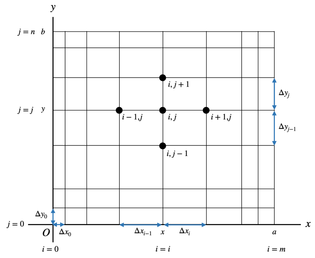
Label the grid points in the $x$ direction as $i=0 \sim m$ and in the $y$ direction as $j=0 \sim n$. Label the point $(x,y)$ on the grid as $(i,j)$ and the value of $u$ at this point as $u_{i,j}$. Label the neighboring grid points as shown in the figure with $\Delta x_i,\Delta y_i$, etc. The difference approximations for partial derivatives $∂u/∂x, ∂u/∂y$ can be represented as follows, fixing $j$ for $∂u/∂x$ and $i$ for $∂u/∂y$.
For forward difference approximation:
$$
\begin{aligned}
\frac{∂u}{∂x} = \frac{u_{i+1, j} – u_{i, j}}{\Delta x_i} \\
\frac{∂u}{∂y} = \frac{u_{i, j+1} – u_{i, j}}{\Delta y_i}
\end{aligned}
$$
For backward difference approximation:
$$
\begin{aligned}
\frac{∂u}{∂x} = \frac{u_{i, j} – u_{i-1, j}}{\Delta x_i} \\
\frac{∂u}{∂y} = \frac{u_{i, j} – u_{i, j-1}}{\Delta y_i}
\end{aligned}
$$
For central difference approximation:
$$
\begin{aligned}
\frac{∂u}{∂x} = \frac{u_{i+1, j} – u_{i-1, j}}{\Delta x_{i-1} + \Delta x_i} \\
\frac{∂u}{∂y} = \frac{u_{i, j+1} – u_{i, j-1}}{\Delta y_{i-1} + \Delta y_i}
\end{aligned}
$$
The second-order partial derivatives, for example using central difference approximation for $∂^2u / ∂x∂y$, are represented as follows:
$$
\frac{∂^2u}{∂x∂y}=\frac{∂}{∂x}
\Big( \frac{∂u}{∂y} \Big) =\frac{(∂u/∂y)_{i+1,j} – (∂u/∂y)_{i-1,j}}{\Delta x_{i-1} + \Delta x_{i}}
$$
$(∂u/∂y)_{i+1,j}$ is obtained by fixing $i+1$ and taking the (central) difference of $u$:
$$
\Big( \frac{∂u}{∂y} \Big)_{i+1,j} = \frac{u_{i+1,j+1} – u_{i+1,j-1}}{\Delta y_{i-1} + \Delta y_{i}}
$$
Similarly, for $(∂u/∂y)_{i-1,j}$ by fixing $i-1$:
$$
\Big( \frac{∂u}{∂y} \Big)_{i-1,j} = \frac{u_{i-1,j+1} – u_{i-1,j-1}}{\Delta y_{i-1} + \Delta y_{i}}
$$
Therefore:
$$
\frac{∂^2u}{∂x∂y}=\frac{u_{i+1, j+1} – u_{i+1, j-1} – u_{i-1, j+1} + u_{i-1, j-1}}{(\Delta x_{i-1} + \Delta x_{i})(\Delta y_{i-1} + \Delta y_{i})}
$$
For $∂^2u/∂x^2$ and $∂^2u/∂y^2$, using forward difference for $∂u/∂x$ and $∂u/∂y$:
$$
\frac{∂^2u}{∂x^2}=\frac{∂}{∂x}
\Big( \frac{∂u}{∂x} \Big) =\frac{(∂u/∂x)_{i+1,j} – (∂u/∂x)_{i,j}}{\Delta x_{i}}
$$
Using backward difference for $(∂u/∂x)_{i+1,j}$ and $(∂u/∂x)_{i,j}$:
$$
\Big( \frac{∂u}{∂x} \Big)_{i+1,j} = \frac{u_{i+1,j} – u_{i,j}}{\Delta x_{i}}, \ \ \ \ \ \ \Big( \frac{∂u}{∂x} \Big)_{i,j} = \frac{u_{i,j} – u_{i-1,j}}{\Delta x_{i-1}}
$$
Then:
$$
\frac{∂^2u}{∂x^2}=\Big(
\frac{u_{i+1,j} – u_{i,j}}{\Delta x_{i}}
–
\frac{u_{i,j} – u_{i-1,j}}{\Delta x_{i-1}}
\Big) \Big/ \Delta x_{i}
$$
Similarly, for $∂^2u/∂y^2$:
$$
\frac{∂^2u}{∂y^2}=\Big(
\frac{u_{i,j+1} – u_{i,j}}{\Delta y_{i}}
–
\frac{u_{i,j} – u_{i,j-1}}{\Delta y_{i-1}}
\Big) \Big/ \Delta y_{i}
$$
If the grid spacing is uniform:
$$
\begin{aligned}
\Delta x_{i-1} = \Delta x_{i} =h \\
\Delta y_{i-1} = \Delta y_{i} =k \end{aligned}
$$
Then, replace the above equations with $h$ and $k$. The results using central difference are as follows:
$$
\begin{aligned}
\frac{∂u}{∂x} = \frac{1}{2h}(u_{i+1,j} – u_{i-1,j}) \\
\frac{∂u}{∂y} = \frac{1}{2k}(u_{i,j+1} – u_{i,j-1})
\end{aligned}
$$
Second-order partial derivatives are as follows:
$$
\begin{align*}
\frac{∂^2u}{∂x∂y} &= \frac{1}{4hk}(u_{i+1,j+1} – u_{i+1,j-1} – u_{i-1,j+1} + u_{i-1,j-1}) \\
\frac{∂^2u}{∂x^2} &= \frac{1}{h^2}(u_{i+1,j} – 2u_{i,j} + u_{i-1,j}) \\
\frac{∂^2u}{∂y^2} &= \frac{1}{k^2}(u_{i,j+1} – 2u_{i,j} + u_{i,j-1})
\end{align*}
$$
Overview of Numerical Solution using the Finite Difference Method
The steps for numerically solving a partial differential equation using the finite difference method are:
1. Convert the partial differential equation into a difference equation.
2. Calculate the values of each element using the difference equation.
Let’s explain each step below.
Converting Partial Differential Equations to Difference Equations
Consider solving the Laplace equation
$$
\frac{∂^2u}{∂x^2} + \frac{∂^2u}{∂y^2} = 0; \ \ \ \ \ \ 0 \leqq x \leqq a, 0 \leqq y \leqq b \ \ \ \ (1)
$$
under the boundary conditions
$$
u(0,y) = p(y), \ \ \ u(a,y) = q(y) \\
u(x,0) = v(x), \ \ \ u(x,b) = w(x)
$$
($a, b, p,q,v,w$ are known).
First, let’s express equation $(1)$ as a difference equation using the difference approximations for partial derivatives discussed in the previous section:
$$
\frac{(u_{i+1,j} – 2u_{i,j} + u_{i-1,j}) }{h^2} + \frac{(u_{i,j+1} – 2u_{i,j} + u_{i,j-1}) }{k^2} = 0
$$
From this, $u_{i,j}$ can be expressed as:
$$
u_{i,j}=\frac{1}{2(h^2+k^2)} \{k^2(u_{i+1,j} + u_{i-1,j}) + h^2(u_{i,j+1} + u_{i,j-1})\} \ \ \ \ (2)
$$
Calculating Each Element’s Value Using the Difference Equation
Let’s take a closer look at the difference equation for $u_{i,j}$.
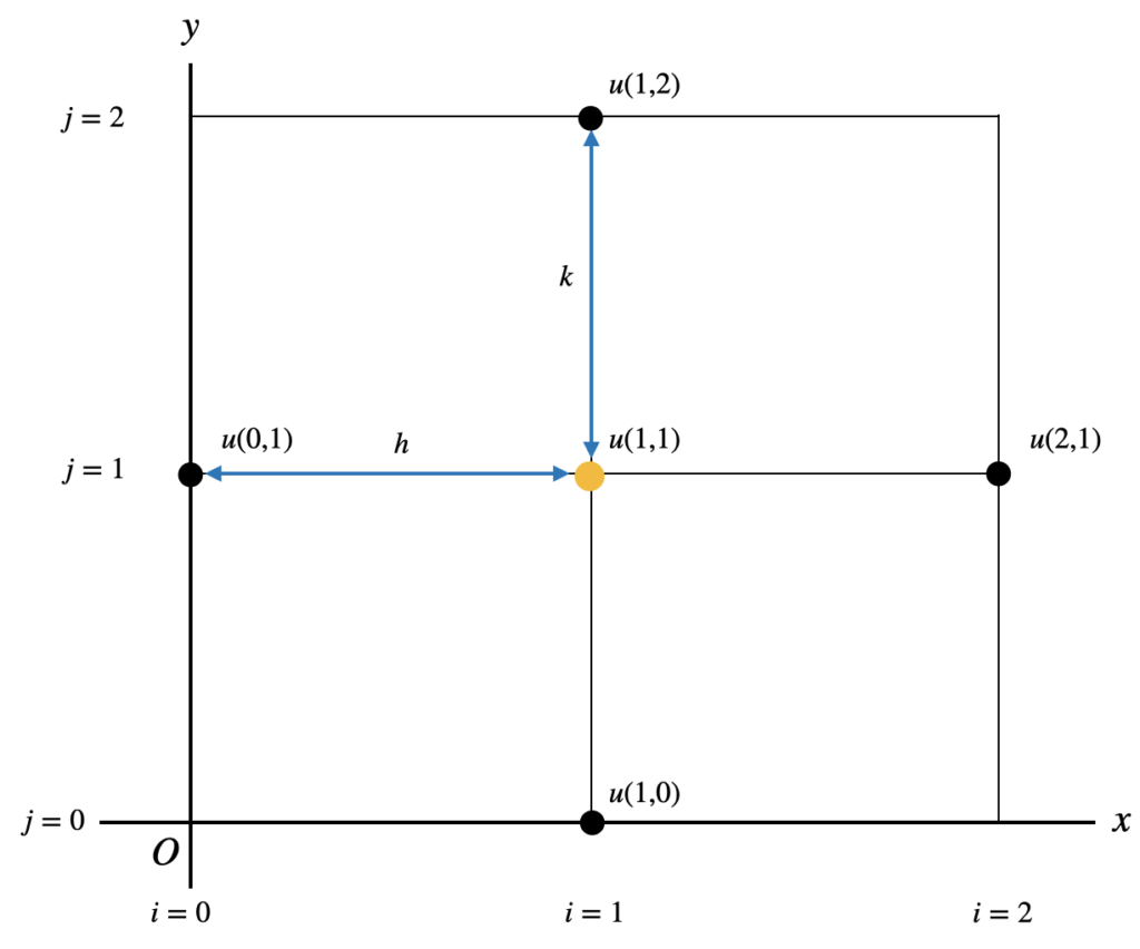
For example, to calculate $u_{1,1}$, using equation $(2)$:
$$
u_{1,1}=\frac{1}{2(h^2+k^2)} \{k^2(u_{2,1} + u_{0,1}) + h^2(u_{1,2} + u_{1,0})\}
$$
As shown in the figure below, if $u_{2,1}, u_{0,1}, u_{1,2}, u_{1,0}$ are known, then $u_{1,1}$ can be calculated. The value of $u$ at a grid point can be calculated from the $u$ values of the surrounding grid points.
The values of $u$ on the boundary $p(y),q(y),v(x),w(x)$ are known, so for the other $u_{i,j}(i=1,2, …, m-1;j=1,2, …, n-1)$, assign an initial value, such as $u_{i,j}=0$, and substitute this initial value into equation $(2)$ to calculate the new $u_{i,j}^{(1)}$. Then, substitute $u_{i,j}^{(1)}$ into $(2)$ to calculate the next value $u_{i,j}^{(2)}$. Repeat this process until the relative error between the $k$th and $(k+1)$th approximation values is smaller than a sufficiently small $\epsilon$, i.e.,
$$
|(u_{i,j}^{(k+1)} – u_{i,j}^{(k)}) / u_{i,j}^{(k+1)}| \leqq \epsilon; \ \ \ \ i=1,2, …, m-1; \ \ j=1,2, …, n-1;
$$
When this condition is met, the solution is considered converged, and $u_{i,j}^{(k+1)}$ is taken as the solution. However, as the number of grid points increases, the number of solutions $u_{i,j}$ to be determined increases, and convergence determination takes time.
One method to reduce the time for convergence determination is to simultaneously determine the convergence of all solutions. This means using the total relative amount of error to determine convergence:
$$
\sum_{i=1}^{m-1}\sum_{j=1}^{n-1} \Big|u_{i,j}^{(k+1)} – u_{i,j}^{(k)} \Big| \Big/ \sum_{i=1}^{m-1}\sum_{j=1}^{n-1}\Big|u_{i,j}^{(k+1)}\Big| \leqq \epsilon
$$
Moreover, when performing iterative calculations using equation $(2)$, using the most recent value of $u$ accelerates convergence. Therefore, when calculating the $(k+1)$th approximation solution, if $u_{i,j}^{(k+1)}$ has already been calculated, use that value. Consequently, the iterative formula in equation $(2)$ is expressed as follows:
$$
u_{i,j}^{(k+1)}=\frac{1}{2(h^2+k^2)} \{k^2(u_{i+1,j}^{(k)} + u_{i-1,j}^{(k+1)}) + h^2(u_{i,j+1}^{(k)} + u_{i,j-1}^{(k+1)})\} \ \ \ \ (3)
$$
This iterative method using equation $(3)$ is known as the Gauss-Seidel method. This article introduces a numerical solution using the Gauss-Seidel method in the example below.
Example Problem
Consider a square plate with each side of length $1$, where the temperature on three sides is maintained at $0$ and the remaining side at a temperature of $f(x)=4x(1-x)$. Determine the temperature distribution within the plate.
The fundamental equation for this problem is the two-dimensional Laplace equation (where $u(x,y)$ represents temperature), shown below along with the boundary conditions:
$$
\frac{∂^2u}{∂x^2} + \frac{∂^2u}{∂y^2} = 0; \ \ \ \ \ \ 0 \leqq x \leqq 1, 0 \leqq y \leqq 1
$$
$$
u(0,y) = 0, \ \ \ u(1,y) = 0 \\
u(x,0) = 0, \ \ \ u(x,1) = 4x(1-x)
$$
Labeling grid points as $i=0 \sim m, j=0 \sim n$ and the value of $u$ at any grid point as $u_{i,j}$.
As introduced above, first, we convert this partial differential equation into a difference equation, and then we implement a program to solve the difference equation.
Implementation Method
The code can be implemented as follows:
The creation of graphs and output to text files is also included, making the code somewhat lengthy, but the crucial part is the calculate_equation function.
Save the following implementation as main.py in a folder (here, ~/Desktop/labcode/python/numerical_calculation/elliptic_equation).
import matplotlib.pyplot as plt
import numpy as np

def _set_initial_condition(
    *,
    array_2d: list,
    grid_counts_x: int,
    grid_counts_y: int,
) -> None:
    """
    Set initial conditions

    Set all U values except for the boundary to 0.0001
    """
    for j in range(1, grid_counts_y):
        for i in range(1, grid_counts_x):
            array_2d[i][j] = 0.0001

def _set_boundary_condition(
    *,
    array_2d: list,
    grid_counts_x: int,
    grid_counts_y: int,
    grid_space: float,
) -> None:
    """Set boundary conditions"""
    # Boundary condition on y=0
    for i in range(grid_counts_x + 1):
        array_2d[i][0] = 0.0

    # Boundary condition on y=M
    for i in range(grid_counts_x + 1):
        array_2d[i][grid_counts_y] = 4 * (grid_space * i) * (1.0 - grid_space * i)

def _is_converged(*, U: list, UF: list, M: int, N: int) -> bool:
    """
    Perform convergence check

    If the total relative error is below ERROR_CONSTANT, it is considered converged
    """
    ERROR_CONSTANT: float = 0.0001  # Precision constant
    sum: float = 0.0  # Initial error value
    sum0: float = 0.0

    for j in range(1, N):
        for i in range(1, M):
            sum0 += abs(U[i][j])
            sum += abs(U[i][j] - UF[i][j])

    sum = sum / sum0
    return sum <= ERROR_CONSTANT

def calculate_equation(*, M: int, N: int, H: float, MK: int) -> (list, int):
    """
    Calculate the difference equation

    The core function of this program
    """
    # List for U values
    U: list = [[0.0 for _ in range(M + 1)] for _ in range(N + 1)]
    # List for U values (for accuracy check)
    UF: list = [[0.0 for _ in range(M + 1)] for _ in range(N + 1)]

    # Set initial values
    _set_initial_condition(
        array_2d=U,
        grid_counts_x=M,
        grid_counts_y=N,
    )
    _set_boundary_condition(
        array_2d=U,
        grid_counts_x=M,
        grid_counts_y=N,
        grid_space=H,
    )

    # Calculation
    calc_count: int = 0
    for _ in range(MK):
        for j in range(1, N):
            for i in range(1, M):
                UF[i][j] = U[i][j]  # Copy U to UF for convergence check
                U[i][j] = (U[i + 1][j] + U[i - 1][j] + U[i][j + 1] + U[i][j - 1]) / 4.0
        calc_count += 1

        # Check for convergence
        if _is_converged(U=U, UF=UF, M=M, N=N):
            print("Converged")
            break
    return U, calc_count

def color_plot(
    *,
    array_2d: list,
    grid_counts: int,
    grid_space: float,
) -> None:
    """
    2D color plot

    When plotting array_2d as is with imshow, the origin is top-left, x-axis is rightward, and y-axis is downward.
    To plot array_2d with x-axis and y-axis correctly, transpose it and use origin="lower" to make the y-axis upward.
    """
    # Specify the range for the axes
    min_x_y = 0.0 - grid_space / 2
    max_x_y = grid_space * grid_counts + grid_space / 2
    extent = (min_x_y, max_x_y, min_x_y, max_x_y)

    # Transpose the 2D array
    array_2d = np.array(array_2d).T
    plt.imshow(
        array_2d,
        cmap="viridis",
        interpolation="none",
        aspect="auto",
        origin="lower",
        extent=extent,
    )
    plt.colorbar()
    plt.savefig("./2d_color_plot.png", format="png")

def output_result_file(
    array_2d: list,
    grid_counts_x: int,
    grid_counts_y: int,
    grid_space: float,
    calc_count: int,
) -> None:
    """Write a 2D array to a text file"""
    with open("./calculated_result.txt", "w") as file:
        file.write(f"# This file shows calculated result as below.\n\n")
        file.write(f"# Calculation Parameters.\n")
        file.write(f"grid_counts_x: {grid_counts_x}\n")
        file.write(f"grid_counts_y: {grid_counts_y}\n")
        file.write(f"grid_space: {grid_space}\n")
        file.write(f"calculation_count: {calc_count}\n\n")

        file.write(f"# Calculated Matrix H.\n")
        for row in array_2d:
            line = " ".join(map(str, row))
            file.write(line + "\n")

if __name__ == "__main__":
    """
    Numerical solution of elliptic equations (Gauss-Seidel method)

    Implemented with the assumption that grid_counts_x = grid_counts_y
    The grid space is the interval, where grid_space = 1 / grid_counts_x
    """
    grid_counts_x: int = 10  # Value of grid point number m
    grid_counts_y: int = 10  # Value of grid point number n
    grid_space: float = 0.1  # Interval
    total_calc_count: int = 1000  # Total calculation count

    array_2d, calc_count = calculate_equation(
        M=grid_counts_x,
        N=grid_counts_y,
        H=grid_space,
        MK=total_calc_count,
    )
    color_plot(
        array_2d=array_2d,
        grid_counts=grid_counts_x,
        grid_space=grid_space,
    )
    output_result_file(
        array_2d=array_2d,
        grid_counts_x=grid_counts_x,
        grid_counts_y=grid_counts_y,
        grid_space=grid_space,
        calc_count=calc_count,
    )
Executing the Program
Open the terminal and enter:
$ cd Desktop/labcode/python/numerical_calculation/elliptic_equationThen, execute the following command (ignore the $ symbol):
$ python main.pyExecution Results
If a file named 2d_color_plot.png is created in ~/Desktop/LabCode/python/numerical_calculation/elliptic_equation and it looks like the following, you have succeeded!
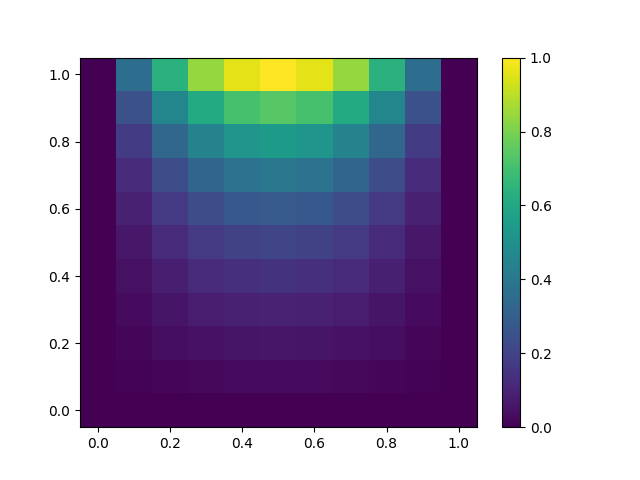
The gradual spread of temperature from the boundary is visualized. On the boundary at $y=1$, the temperature distribution is based on $4x(1-x)$, and the distribution elsewhere is based on the Laplace equation. In this Fig., what appears as mass should be understood as grid points.
Additionally, a text file named calculated_result.txt should be created as follows. Although only basic information is output here, by outputting both the calculation results and the parameters used, the calculation results can be evaluated by others. It’s good practice to output results for both your and others’ benefit.
# This file shows calculated result as below.

# Calculation Parameters.
grid_counts_x: 10
grid_counts_y: 10
grid_space: 0.1
calculation_count: 70

# Calculated Matrix H.
0.0 0.0 0.0 0.0 0.0 0.0 0.0 0.0 0.0 0.0 0.0
0.0 0.008929031616324612 0.018753985587845273 0.03045645155113031 0.045215630200268656 0.06454923902703041 0.09052691584655263 0.12614272692516448 0.176072856491503 0.24847942773093906 0.36000000000000004
0.0 0.01698198799554465 0.03566140261199987 0.05789421689302395 0.0858976328737752 0.12249382757113862 0.17145009762302302 0.23799771175707277 0.32968623257237084 0.4578514986882389 0.6400000000000001
0.0 0.023368460401624713 0.04906242166685223 0.07961842109132274 0.11804753163349524 0.1681365089053069 0.23483228099737163 0.3247502516018773 0.44684690227830404 0.6132490318574787 0.8400000000000001
0.0 0.02746745619852549 0.057658441258696666 0.0935383066055323 0.1386104193192113 0.19724196923107878 0.27505222681215186 0.3793696506354582 0.519730238272764 0.708307450428056 0.96
0.0 0.02888372196913288 0.060626251326013327 0.09833879795793664 0.14569078617968717 0.20724196857771687 0.28882793868670115 0.3979934782131962 0.5444261214543008 0.7402602555170518 1.0
0.0 0.02748059290857848 0.05768220659138331 0.09356941707013768 0.1386452033228391 0.19727675460305522 0.27508369154227 0.37939510680256094 0.5197478283548784 0.7083162455407579 0.96
0.0 0.023390838059342566 0.04910290459911079 0.07967141605927938 0.11810678428463689 0.16819576389806784 0.23488587946502332 0.3247936148115438 0.4468768660372461 0.6132640138588368 0.8399999999999999
0.0 0.017006426661918712 0.03570561407859771 0.05795209278737131 0.0859623428147862 0.12255854008880909 0.1715086326507498 0.238045068840605 0.3297189560804824 0.45786786057508466 0.6399999999999999
0.0 0.008946212816146909 0.01878506773578349 0.030497140267083136 0.045261123502502935 0.06459473415967246 0.09056806800477205 0.12617602060802796 0.1760958622623825 0.2484909307093668 0.35999999999999993
0.0 0.0 0.0 0.0 0.0 0.0 0.0 0.0 0.0 0.0 0.0
Code Explanation
This Python code deals with the numerical solution of elliptic equations, calculating approximate solutions under specific conditions and outputting the results as graphs and text files. The code is divided into several key parts as described below:
1. Main Execution Block in Python
if __name__ == "__main__":
    """
    Numerical solution of elliptic equations (Gauss-Seidel method)

    Implemented assuming grid_counts_x = grid_counts_y
    grid_space is the interval, where grid_space = 1 / grid_counts_x
    """
    grid_counts_x: int = 10  # Grid point number m value
    grid_counts_y: int = 10  # Grid point number n value
    grid_space: float = 0.1  # Interval
    total_calc_count: int = 1000  # Total calculation count

    array_2d, calc_count = calculate_equation(
        M=grid_counts_x,
        N=grid_counts_y,
        H=grid_space,
        MK=total_calc_count,
    )
    color_plot(
        array_2d=array_2d,
        grid_counts=grid_counts_x,
        grid_space=grid_space,
    )
    output_result_file(
        array_2d=array_2d,
        grid_counts_x=grid_counts_x,
        grid_counts_y=grid_counts_y,
        grid_space=grid_space,
        calc_count=calc_count,
    )
This code is written inside the main execution block (if __name__ == "__main__") in Python, forming the essential part of the script that implements the numerical solution of elliptic equations. When a Python program is executed, the code within this execution block runs first.
Here, the process of calculating the numerical solution using the Gauss-Seidel method and outputting the results as plots and files is defined. Each step is explained in detail below.
Workflow
1. Setting Parameters
-
grid_counts_xandgrid_counts_y: Define the differential grid used for calculations. Both are set to 10 here, forming a 10×10 grid, resulting in 11×11 grid points. grid_space: Defines the interval between grid points. Set to 0.1 here, based on the relationshipgrid_space = 1 / grid_counts_x, ensuring a uniform grid interval.total_calc_count: Defines the total number of calculation iterations. In this example, it is set to 1000.
2. Calculating the Numerical Solution
- The
calculate_equationfunction calculates the numerical solution of the elliptic equation using the specified parameters (number of grid points, interval, number of calculations). - This function returns the calculated 2D array (numerical solution) and the actual number of calculations.
3. Visualizing the Results
- The
color_plotfunction visualizes the calculated 2D array as a color plot. - The plot is created based on
array_2d, withgrid_counts_xandgrid_spaceused to set the appropriate axis ranges.
4. Outputting Results to a File
- The
output_result_filefunction outputs the 2D array of results as a text file. - The file includes both the calculation parameters and the results.
2. Calculating the Difference Equation
def calculate_equation(*, M: int, N: int, H: float, MK: int) -> (list, int):
    """
    Calculate the difference equation

    The core function of this program
    """
    # List for U values
    U: list = [[0.0 for _ in range(M + 1)] for _ in range(N + 1)]
    # List for U values (for accuracy determination)
    UF: list = [[0.0 for _ in range(M + 1)] for _ in range(N + 1)]

    # Setting initial values
    _set_initial_condition(
        array_2d=U,
        grid_counts_x=M,
        grid_counts_y=N,
    )
    _set_boundary_condition(
        array_2d=U,
        grid_counts_x=M,
        grid_counts_y=N,
        grid_space=H,
    )

    # Calculation process
    calc_count: int = 0
    for _ in range(MK):
        for j in range(1, N):
            for i in range(1, M):
                UF[i][j] = U[i][j]  # Copy U to UF for convergence check
                U[i][j] = (U[i + 1][j] + U[i - 1][j] + U[i][j + 1] + U[i][j - 1]) / 4.0
        calc_count += 1

        # Convergence check
        if _is_converged(U=U, UF=UF, M=M, N=N):
            print("Converged")
            break
    return U, calc_count
The calculate_equation function calculates the numerical solution of the difference equation, employing a common method used in solving elliptic equations. The key aspects and operations of this function are explained below.
1. Parameters
MandN: Specify the number of grid points along the X and Y axes, respectively.H: Indicates the interval, defining the spatial interval between grid points.MK: Specifies the maximum number of calculations.
2. Initializing Variables
U: A 2D array storing the solution. Initially, all values are set to 0.0.UF: A 2D array of the same size asU, used for accuracy determination.
3. Setting Initial and Boundary Conditions
_set_initial_condition: Sets initial conditions in the arrayU, defining the initial state for a specific problem._set_boundary_condition: Sets boundary conditions in the arrayU, defining the behavior at the spatial boundaries of the problem.
4. Calculation Process
- The calculation repeats
MKtimes. In each iteration, each element of the arrayUis updated to the average value of its adjacent elements. This step represents the discretization of the difference equation, part of the Gauss-Seidel method. - After each iteration,
Uis copied toUF, and a convergence check_is_convergedis performed. The calculation ends if the convergence criteria are met.
5. Convergence Check
_is_converged: This function evaluates the difference between old valuesUFand new valuesU, determining if it is sufficiently small. This confirms whether the numerical solution has stabilized.
6. Returning Results
- Finally, the function returns the 2D array
U(calculated solution) and the actual number of calculationscalc_count.
3. Plotting 2D Array Data
def color_plot(
    *,
    array_2d: list,
    grid_counts: int,
    grid_space: float,
) -> None:
    """
    2D color plot

    Plotting array_2d as is with imshow results in the origin being top-left, x-axis rightward, and y-axis downward.
    To plot array_2d correctly with x and y axes, it is transposed and then plotted with origin="lower" to make the y-axis upward.
    """
    # Specify the axes range
    min_x_y = 0.0 - grid_space / 2
    max_x_y = grid_space * grid_counts + grid_space / 2
    extent = (min_x_y, max_x_y, min_x_y, max_x_y)

    # Transpose the 2D array
    array_2d = np.array(array_2d).T
    plt.imshow(
        array_2d,
        cmap="viridis",
        interpolation="none",
        aspect="auto",
        origin="lower",
        extent=extent,
    )
    plt.colorbar()
    plt.savefig("./2d_color_plot.png", format="png")
The color_plot function visualizes data from a 2D array as a color plot, particularly useful for illustrating results from numerical simulations or analyses. The main features of the function are explained below.
1. Parameters
array_2d: The 2D array containing data to be visualized.grid_counts: Specifies the number of grids, indicating the size of the array along the X and Y axes.grid_space: The spatial interval between grids (interval).
2. Specifying Axes Range
min_x_yandmax_x_y: Determine the range of the graph’s X and Y axes.extent: A parameter passed to theimshowfunction, specifying the display range of the image.
3. Transposing the 2D Array
array_2d = np.array(array_2d).T: Transposes the 2D array, swapping its rows and columns to display correctly in the conventional Cartesian coordinate system.
4. Generating a Color Plot
plt.imshow: Uses matplotlib’simshowfunction to display the 2D data as an image.cmap="viridis": Sets the color map toviridis, a popular color map that represents data changes with color.interpolation="none": No interpolation is applied to the image.aspect="auto": Automatically adjusts the aspect ratio of the image.origin="lower": Sets the image’s origin to the bottom left.extent=extent: Sets the display range of the image.
5. Adding a Color Bar and Saving
plt.colorbar(): Adds a color bar to display the color scale corresponding to the data values.plt.savefig("./2d_color_plot.png", format="png"): Saves the graph as a PNG file.
4. Outputting Results to a File
def output_result_file(
    array_2d: list,
    grid_counts_x: int,
    grid_counts_y: int,
    grid_space: float,
    calc_count: int,
) -> None:
    """Write a 2D array to a text file"""
    with open("./calculated_result.txt", "w") as file:
        file.write(f"# This file shows calculated result as below.\n\n")
        file.write(f"# Calculation Parameters.\n")
        file.write(f"grid_counts_x: {grid_counts_x}\n")
        file.write(f"grid_counts_y: {grid_counts_y}\n")
        file.write(f"grid_space: {grid_space}\n")
        file.write(f"calculation_count: {calc_count}\n\n")

        file.write(f"# Calculated Matrix H.\n")
        for row in array_2d:
            line = " ".join(map(str, row))
            file.write(line + "\n")
The output_result_file function is used to output data from a calculated 2D array to a text file, particularly useful for saving results from numerical simulations or analyses. The operation of the function is explained below.
1. Creating and Writing to the File
with open("./calculated_result.txt", "w") as file: This statement creates a new text file namedcalculated_result.txtin the current directory and opens it in write mode. Using thewithstatement ensures that the file is automatically closed after the file operations are completed.
2. Writing Calculation Parameters
- The function first writes information about the parameters used for the calculation (
grid_counts_x,grid_counts_y,grid_space,calc_count) to the file. This documents the information necessary for analyzing and reproducing the data.
3. Writing the Calculated Data
- Next, it writes each row of the 2D array stored in
array_2d(here, the calculated matrix H) to the text file. for row in array_2d: This loop iterates over each row of the array.line = " ".join(map(str, row)): Converts each element of the row (a number) to a string, joins them with spaces into one string.file.write(line + "\\n"): Writes the converted string to the file, inserting a newline after each row to start the next row on a new line.
5. Other Functions
def _set_initial_condition(
    *,
    array_2d: list,
    grid_counts_x: int,
    grid_counts_y: int,
) -> None:
    """
    Set initial conditions

    Set all U values except for the boundary to 0.0001
    """
    for j in range(1, grid_counts_y):
        for i in range(1, grid_counts_x):
            array_2d[i][j] = 0.0001

def _set_boundary_condition(
    *,
    array_2d: list,
    grid_counts_x: int,
    grid_counts_y: int,
    grid_space: float,
) -> None:
    """Set boundary conditions"""
    # Boundary condition on y=0
    for i in range(grid_counts_x + 1):
        array_2d[i][0] = 0.0

    # Boundary condition on y=M
    for i in range(grid_counts_x + 1):
        array_2d[i][grid_counts_y] = 4 * (grid_space * i) * (1.0 - grid_space * i)

def _is_converged(*, U: list, UF: list, M: int, N: int) -> bool:
    """
    Perform convergence check

    If the total relative error is below ERROR_CONSTANT, it is considered converged
    """
    ERROR_CONSTANT: float = 0.0001  # Precision constant
    sum: float = 0.0  # Initial error value
    sum0: float = 0.0

    for j in range(1, N):
        for i in range(1, M):
            sum0 += abs(U[i][j])
            sum += abs(U[i][j] - UF[i][j])

    sum = sum / sum0
    return sum <= ERROR_CONSTANT
These code snippets define functions for setting initial and boundary conditions, as well as for performing convergence checks, particularly in the analysis and solution of partial differential equations. These functions play a crucial role in the numerical analysis process.
_set_initial_condition function
Purpose
- Sets initial conditions in a 2D array (typically a
matrix of grid points used in numerical analysis).
Operation
array_2d: The 2D array used in the analysis.grid_counts_xandgrid_counts_y: The number of grid points along the X and Y axes.- Sets all values in the array (except for the boundary) to
0.0001.
_set_boundary_condition function
Purpose
- Sets specific conditions on the boundary of the 2D array.
Operation
- Sets all values on the
y=0boundary (the bottom row) to0.0. - Sets values on the
y=Mboundary (the top row) according to the formula4 * (grid_space * i) * (1.0 - grid_space * i), wheregrid_spaceindicates the interval between grid points.
_is_converged function
Purpose
- Determines whether the numerical solution method has converged.
Operation
U: The array at the current calculation step.UF: The array at the previous calculation step.MandN: The number of grid points along the X and Y axes.- Calculates the difference between each element of
UandUF, taking the sum of the absolute values. - If this sum is sufficiently small compared to the total sum
sum0(belowERROR_CONSTANT), it is considered converged.
In Conclusion
We have introduced the numerical solution of partial differential equations using the finite difference method.
The Python computation program is also generously shared, so please deepen your understanding by running it.
In the future, we will write new articles on numerically solving other types of partial differential equations, so we hope you will look forward to them.