【scRNA-seq】 How to Start scRNA-seq Analysis Using Seurat (Part 1)【Seurat】

Single-cell RNA sequencing (scRNA-seq) is gaining attention as a method to conduct RNA-seq analysis on individual cell populations.

In this post, we’ll be diving into a hands-on tutorial of Seurat, an R package for scRNA-seq. This is a preparatory step for those who are looking to get started with scRNA-seq.

Since this article follows the Seurat hands-on guide, it’ll help you grasp an overview of how to use Seurat. I encourage you to give it a try!

Tested Environment

macOS Monterey (12.4), Quad-Core Intel Core i7, Memory 32GB

What is Seurat?

Seurat is an R package designed for scRNA-seq data analysis. With Seurat, you can perform tasks such as normalizing scRNA-seq data and visualizing results.

The creators of Seurat have provided a hands-on tutorial. Engaging with it can deepen your understanding of Seurat. However, for those unfamiliar with R, some parts may be challenging. In this article, we’ll walk through the tutorial with added supplementary explanations to make it more accessible.

Setting up the R Environment

To undertake the Seurat tutorial, you’ll need an environment to run R. Personally, I recommend using RStudio.

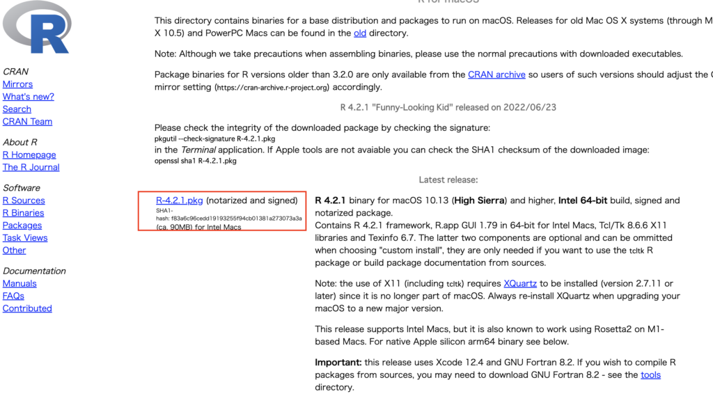
Depending on your OS, please download the installer from this website: https://cran.r-project.org/

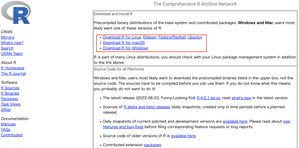
Please select the latest version during installation. The one at the top is the most recent.

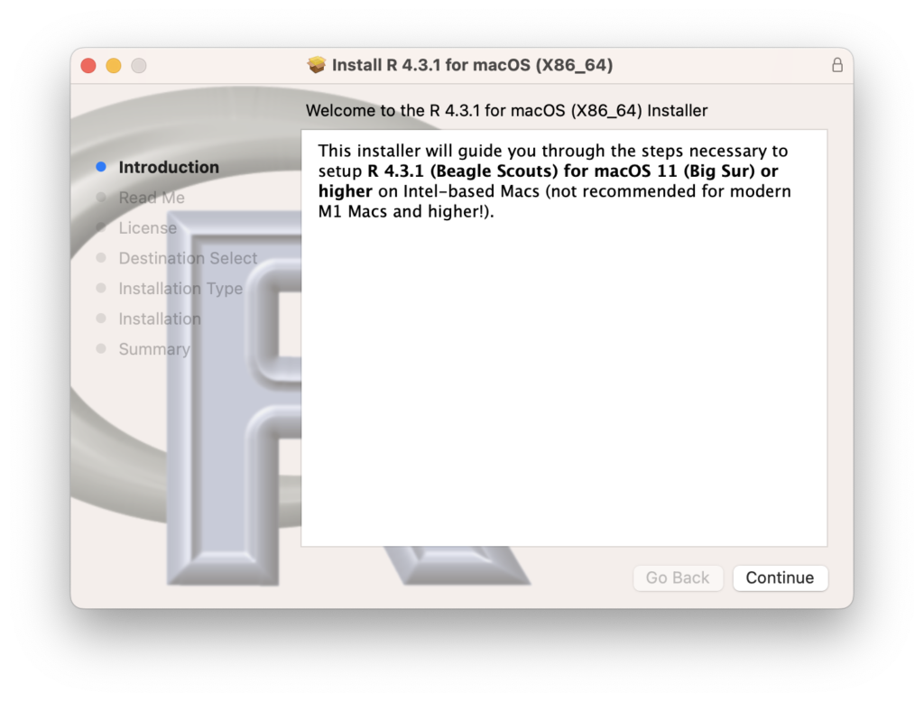
On the installation screen, click “Continue” to complete the process.

Installing RStudio

Navigate to the given URL. As you scroll down a bit, you’ll find a button labeled “DOWNLOAD RSTUDIO.” Please click on it.

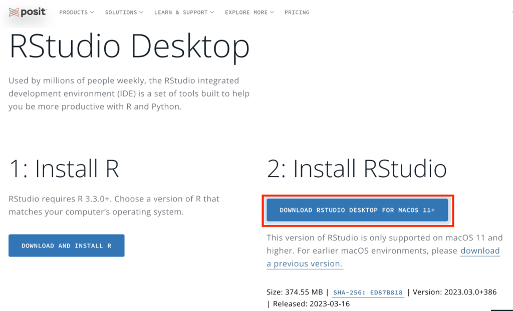
You should be redirected to the following page. Click on the button labeled “2: Install RStudio.” The image shown might be for Mac, but the page will detect your operating system and provide the appropriate RStudio Desktop download. For instance, if you’re using Windows, you’ll be given the Windows version for download. Once downloaded, install it just like you did for R.

Upon launching RStudio, you should see the following interface.

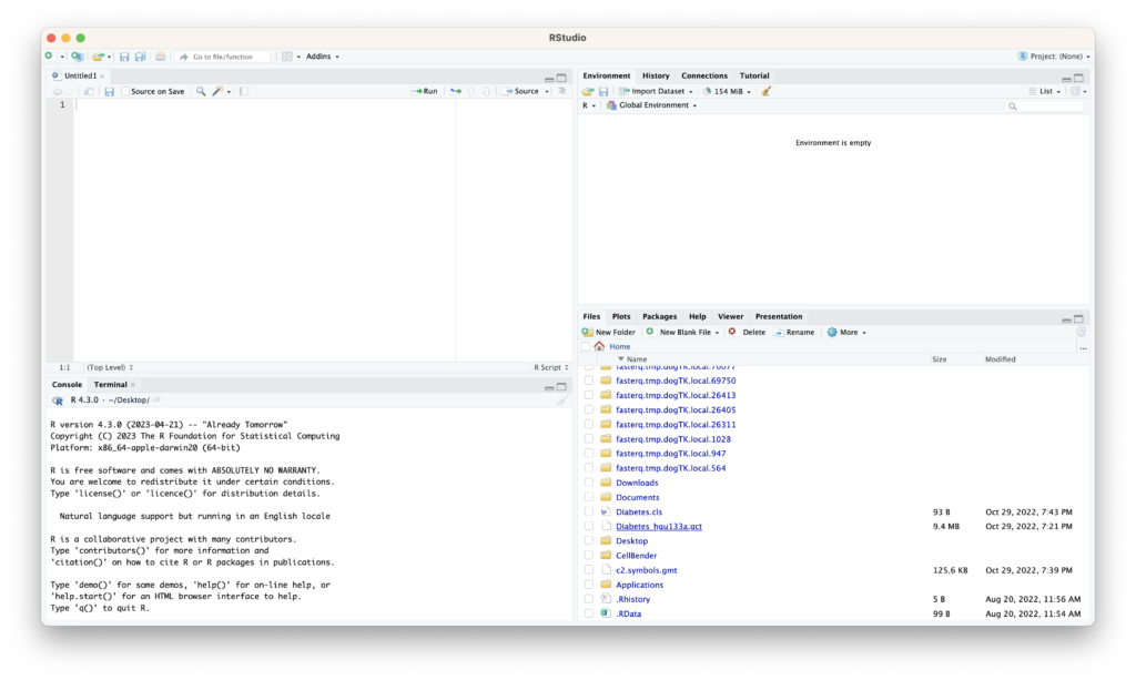
RStudio’s interface is divided into four main panels:

Source Editor (Top-left panel): Here, you can create and edit R scripts or R Markdown files. You can also write R code in this area and execute it by clicking the “Run” button or using shortcut keys (Ctrl+Enter for Windows and Cmd+Enter for Mac).
Console (Bottom-left panel): This is where you can directly execute R code and view the results. It’s also the place to test R commands or view help for functions.
Environment/History (Top-right panel):
- Environment Tab: Displays objects in the workspace (variables, data frames, lists, etc.). New objects will be listed here as they are created.
- History Tab: Shows the history of R commands you’ve executed. It’s a handy feature when you need to reuse past commands.
Files/Plots/Packages/Help (Bottom-right panel):
- Files Tab: Displays files in the working directory.
- Plots Tab: Showcases graphical outputs like plots or charts.
- Packages Tab: Lists installed R packages. You can load packages from here or install new ones.
- Help Tab: Provides documentation for R functions and packages. It’s a valuable resource when you want to check how a particular function works.

Each of these panels operates independently but collaboratively to support R coding. RStudio’s layout is customizable, allowing you to reposition and resize these panels as you see fit.

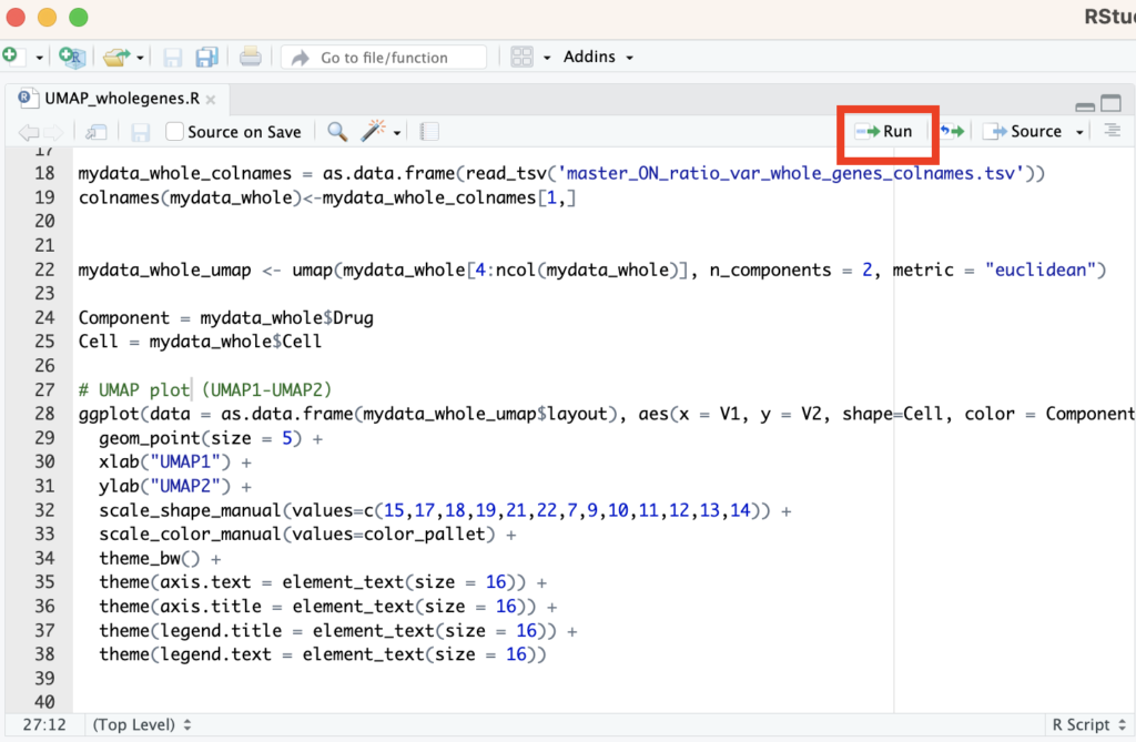
In RStudio, you’ll primarily be writing code in the Source Editor (top-left panel). Remember that clicking “Run” will execute a single line, whereas pressing “Source” will run the entire script.

How to Use Seurat

Preparation for the Hands-On Tutorial

Let’s proceed with Seurat’s hands-on tutorial. First, import the necessary libraries.

install.packages("dplyr")
install.packages("Seurat")
install.packages("patchwork")

Once the installation is complete, follow the instructions below to make the library ready for use.

library(dplyr)
library(Seurat)
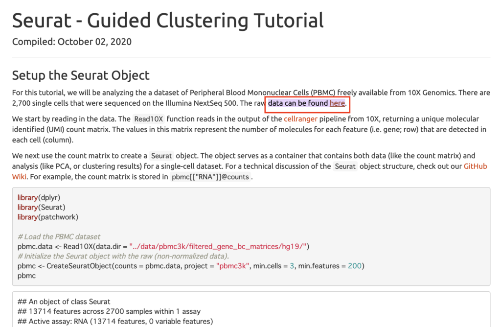
library(patchwork)

Download the raw data from the hands-on site. Access the following link and download from the location marked “here”. [https://satijalab.org/seurat/archive/v3.2/pbmc3k_tutorial.html#:~:text=data%20can%20be%20found%20here]

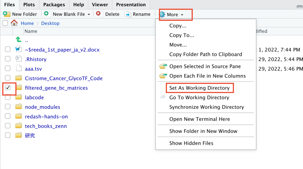
Unzip the downloaded file on your desktop. Then, in the bottom-right window of RStudio, navigate to the desktop and:

Check the downloaded file.
Click “More”.
Select “Set As Working Directory”.

Ensure you do this correctly, as any errors here might prevent subsequent code from running.

Run the command provided below. If you see a path ending with “Desktop”, then you have set it up correctly.

> getwd()
[1] "/Users/[UserName]/Desktop"

Execute the following command to load the data into R. With this, the hands-on preparation is complete.

pbmc.data <- Read10X(data.dir = "./filtered_gene_bc_matrices/hg19/")
pbmc <- CreateSeuratObject(counts = pbmc.data, project = "pbmc3k", min.cells = 3, min.features = 200)
pbmc

Quality Control (QC)

In scRNA-seq, quality control are performed using violin plots to identify cells that might be outliers.

Cells that are dying or of poor quality might exhibit extremely low gene expression levels or show contamination from mitochondria. Additionally, when counting the number of genes, duplicated cells (meaning not single cells) can result in aberrantly high gene counts.

# Using all genes starting with "MT-" as a set of mitochondrial genes
pbmc[["percent.mt"]] <- PercentageFeatureSet(pbmc, pattern = "^MT-")


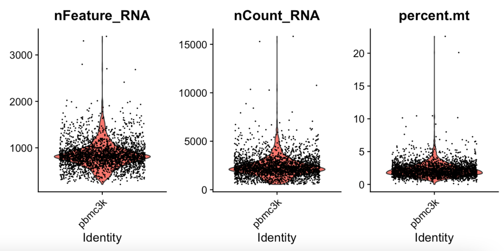
VlnPlot(pbmc, features = c("nFeature_RNA", "nCount_RNA", "percent.mt"), ncol = 3)

Once you input the command, I expect an illustration to appear in the bottom right of RStudio.

Using the cell groups where we can observe bulges in the violin plot, we deduce that these cells provide the most plausible gene count for the entire dataset. Here are the reference values for QC in this sample:

Filter out cells with unique feature counts exceeding 2,500 or below 200, based on nFeature_RNA.
Filter out cells where the mitochondrial count is over 5%, as indicated by percent.mt.

You can employ scatter plots to observe the correlations between these values. Please execute the following code:

plot1 <- FeatureScatter(pbmc, feature1 = "nCount_RNA", feature2 = "percent.mt")
plot2 <- FeatureScatter(pbmc, feature1 = "nCount_RNA", feature2 = "nFeature_RNA")
plot1 + plot2

There doesn’t appear to be a correlation between percent.mt and nCount_RNA (-0.13). However, there is a correlation between nFeature_RNA and nCount_RNA, with a value of 0.95.

Insert the finalized values into the sample pbmc again after QC.

pbmc <- subset(pbmc, subset = nFeature_RNA > 200 & nFeature_RNA < 2500 & percent.mt < 5)

Data Normalization

After removing unnecessary cells from the dataset using QC, the next step is data normalization.

By default, a global scaling normalization method named “LogNormalize” is applied. This method normalizes each cell’s characteristic expression amount by its total expression, multiplies it by a scaling factor (default is 10,000), and then log-transforms the result. After normalizing the data, again input the finalized values into the sample pbmc.

# LogNormalize
pbmc <- NormalizeData(pbmc, normalization.method = "LogNormalize", scale.factor = 10000)

# Inserting into pbmc again
pbmc <- NormalizeData(pbmc)

If you’ve made it this far, the preprocessing of scRNA-seq data is complete. The subsequent steps will cover visualization techniques for the normalized data.

Extracting Genes with High Variability

We’ll compute subsets within the dataset that exhibit significant inter-cell variability — high expression in some cells, and low in others. By default, it’s set to return a variable count of 2,000 per dataset.

# Use the FindVariableFeatures function to prepare the data
pbmc <- FindVariableFeatures(pbmc, selection.method = "vst", nfeatures = 2000)

# Get the top 10 gene names, retrieve the head
top10 <- head(VariableFeatures(pbmc), 10)

# Plot
plot1 <- VariableFeaturePlot(pbmc)
plot2 <- LabelPoints(plot = plot1, points = top10, repel = TRUE)
plot1 + plot2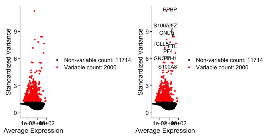

If you encounter an error after inputting the commands…

Should you still face errors after inputting commands correctly, the values you’re trying to input into pbmc might be incorrect. If you come across an error, don’t panic! Go back and re-input the commands from the beginning: Quality Check → Normalization. If you follow the sequence correctly, you should be able to proceed without errors.

For now, I’ll conclude the article here.

The next part can be found in the subsequent article. Do give it a try!