【Autodock Vina】In Silico Screening Using Autodock Vina【In Silico Drug Discovery】

This article is about in silico drug screening using Autodock Vina. In silico drug screening has become a powerful tool for identifying lead compounds from a vast number of small molecules. In this article, we actually perform in silico screening against a protein involved in diabetes and identify potential drug candidate compounds. Since it can be easily done on your own computer, please give it a try!

Tested Environment

Windows 11 Pro (22H2) using Parallels Desktop on a Mac running macOS Ventura (13.2.1). (or a regular Windows ),
OpenBabelGUI(2.3.1)、 MGLTools(1.5.7)　(MGLTools is not compatible with Mac!)
perl 5, version 14, subversion 2 (v5.14.2) built for MSWin32-x86-multi-thread

※Although Parallels Desktop requires a subscription, it allows you to set up a Windows environment on a Mac relatively inexpensively (about 10,000 yen per year) and easily.”

if you’re interested, please give it a try from here. Since you can test Windows just like a regular app without the hassle of setting up a complicated virtual environment, it comes highly recommended.

What is AutoDock Vina？

AutoDock Vina is an open-source software for molecular docking and virtual screening. Its main advantages include:

Speed: Optimized algorithms enable rapid calculations.
Accuracy: As an improved version of AutoDock, it offers high docking precision.
User-friendliness: It employs a simple command-line interface.
Flexibility: Suitable for a wide variety of ligands and target proteins.
Free of charge: Being open-source, it is customizable.
Large-scale screening: Capable of efficiently processing vast compound libraries.
Multi-threading: Supports acceleration using multiple CPU cores.

These features make Vina a potent tool for in silico screening.

What is in silico screening?

identify promising compounds from large molecular libraries against specific biological targets. The term “in silico,” derived from the Latin “in silicium” (in silicon), refers to computer simulations. This process allows for the prediction of structural and biological activity of numerous compounds and the search for the best compounds for a target of interest. It can save time and costs by filtering promising compounds before experimental synthesis and is faster and more comprehensive than experimental screening, thus enhancing drug development efficiency.

In silico screening is used in various fields, including drug discovery, chemical property prediction, and new material design.

Due to computer specifications, it’s challenging to build a large-scale library for this demonstration. Therefore, we will use a small-scale library consisting of three compounds for in silico screening.

Let’s start in silico screening using AutoDock Vina! The steps are as follows:

Preparation of the target protein
Preparation of the compound library
Setting up in silico screening
Conducting in silico screening

Preparation of the Target Protein

We will prepare the target for in silico screening. Many proteins in the Protein Data Bank are in complex with their binders, so we will remove those. We will use DPP4（pdb：2OQV) as an example for this tutorial.

First, open PyMOL and go to File → GetPDB…, enter PDB ID 2OQV, press download, and display DPP4 in PyMOL.

Then, since DPP4 is a protein composed of two identical units, we will specify only one unit.

In PyMOL’s command line, type sele chain A and execute. This command selects the molecule with chain ID A.

sele chain A

Then, to make chain A easily identifiable, execute color red, sele to color it red. Chain A contains a binder, which needs to be removed.

color red, sele

Display the sequence by going to Display → Sequence, select MA9 on the far right, and remove the binder by selecting sele → remove atoms.

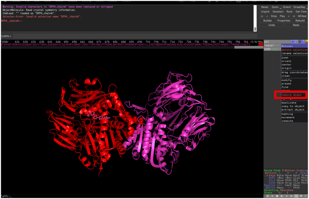
Then, reselect chain A by sele chain A and save it as a PDB file named DPP4_prep.pdb using save DPP4_prep.pdb, sele.

save DPP4_prep.pdb, sele

Next, use MGLTools for further setup.

MGLTools is a software suite that includes molecular modeling and visualization programs. It contains tools used for preprocessing and analyzing results from AutoDock, a free docking software for predicting molecular interactions between proteins and ligands. MGLTools is essential for creating input files for AutoDock and analyzing its outputs. Thus, MGLTools and AutoDock are closely integrated and often used together in complex prediction and drug design research.

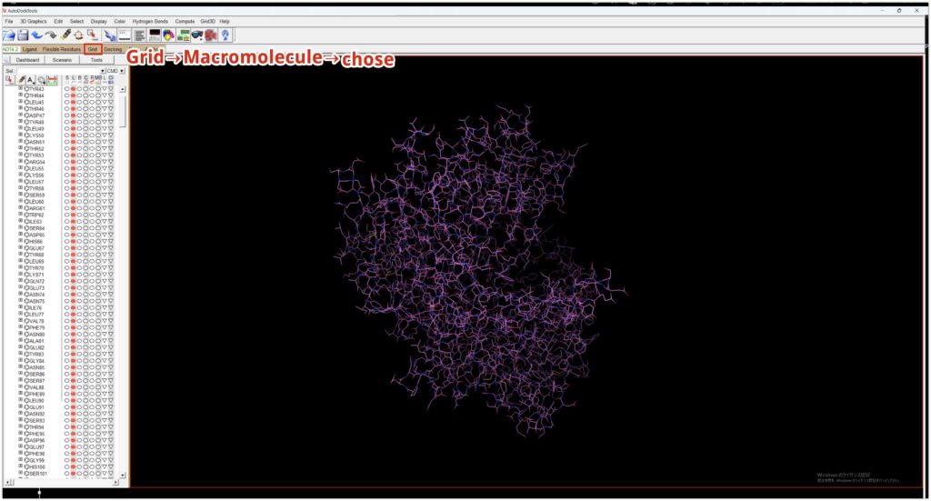
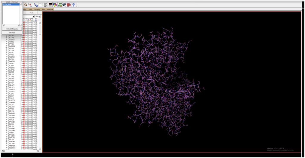
Open MGLTools, go to File → Read Molecule, and open the previously created DPP4_prep.pdb.

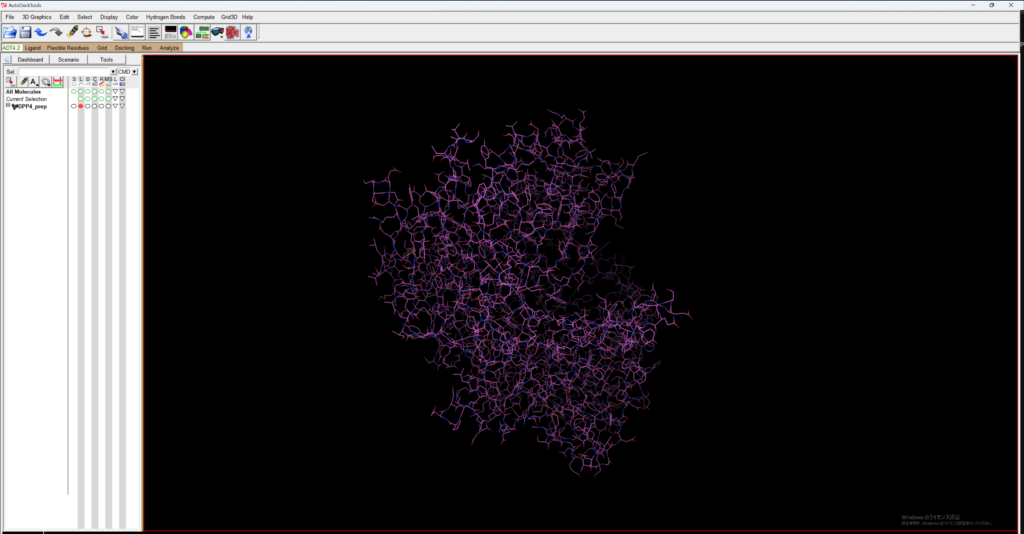
Then, go to Grid → Macromolecule → chose → DPP4_prep to save DPP4_prep as a pdbqt file for AutoDock.

Decide on the binding site for the ligand. Open the previously saved DPP4_prep.pdbqt, and when you open Grid → Gridbox, a box will appear. Since the binding site is unknown, adjust the box to be as large as possible to encompass the protein (although the maximum value is set to 126 here, 80 seems to be a suitable size due to memory considerations).

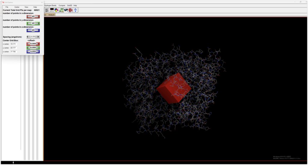
Since the binding site is unknown, adjust the box to be as large as possible to encompass the protein (although the maximum value is set to 126 here, 80 seems to be a suitable size due to memory considerations).

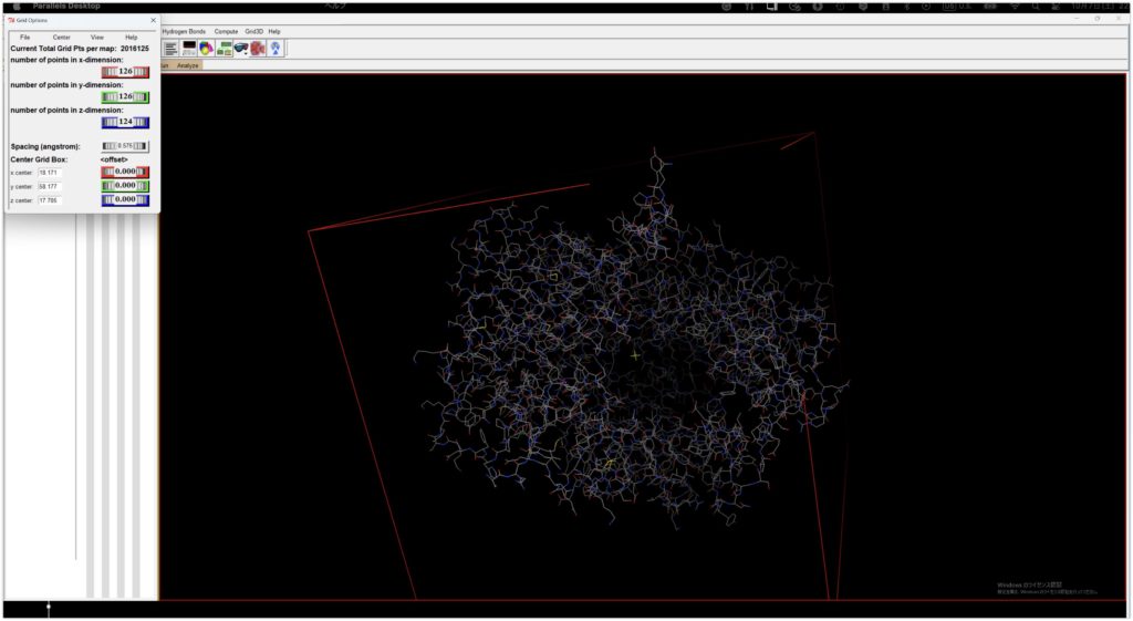
Adjust the Grid Box as shown and save the adjusted Grid Box information for later use by going to Grid Option’s File → Output grid dimensions File.

With this, the protein preparation is complete.

Preparation of the compound library

The ZINC database is a public chemical database used for virtual screening of chemical compounds, providing data and information on chemical compounds to aid in the discovery and design of new drugs. It includes data on various chemical compounds, including chemical structures, physical properties, biological activities, and references, allowing researchers and pharmacists to easily search for and obtain necessary information on various chemical compounds.

The ZINC database is primarily used for virtual screening, a method of rapidly screening vast numbers of chemical compounds on a computer to select promising ones. It is widely used as a valuable tool to support the discovery and design of new drugs through virtual screening.

For a simple compound library, let’s create a small library of three compounds: Omarigliptin, Anagliptin, and ZINC33.

Access the ZINC database , click on the Substances tab, and retrieve the desired small molecule compounds.

Using Omarigliptin as an example, known to act on DPP4, search for Omarigliptin in the search bar, select it, and download the SDF file.

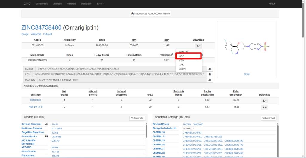
Repeat the process for Anagliptin, which is known to act on DPP4, and ZINC33, an unrelated compound.

Next, convert the SDF files to PDB files using Open Babel, an open-source toolkit for converting and processing chemical information, supporting over 100 chemical data formats, and facilitating data compatibility across different software and databases. Mainly used for converting chemical structure formats, it acts as a “translator” for chemical information.

Download Open Babel version 2.3.1 (note that the latest version, 3.1.1, did not support the output format pdbqt for some reason).

Open OpenBabel, specify the ligand’s SDF file as the input file, choose pdbqt as the OUTPUT FORMAT, and check Add hydrogens (be cautious as not all carbons may have hydrogens attached properly).

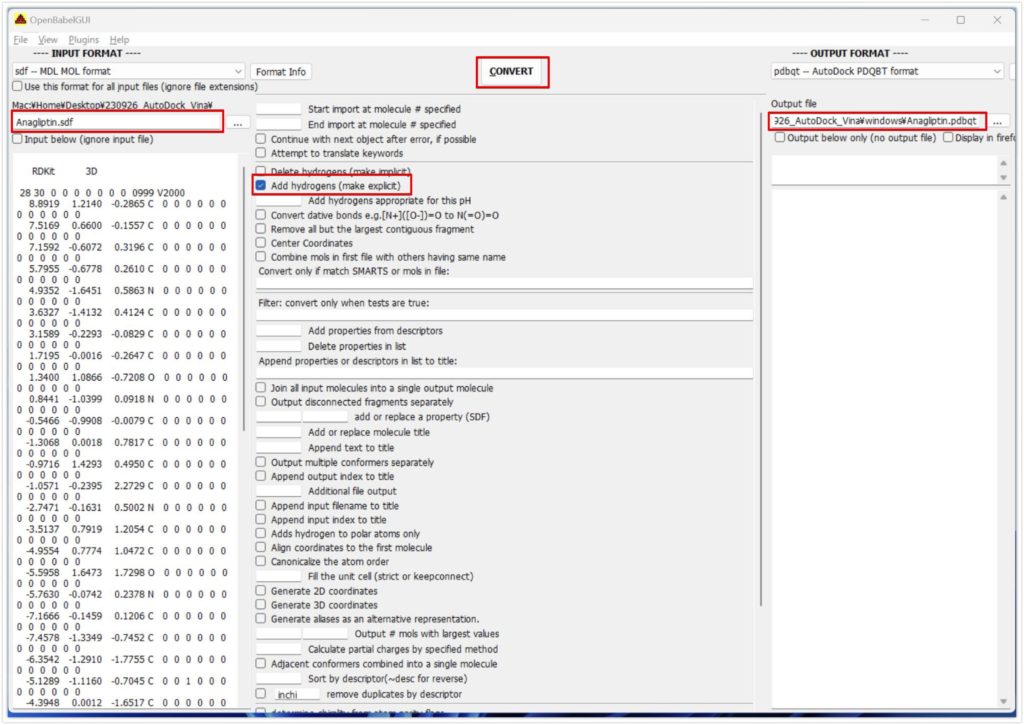
Click Convert to obtain pdbqt files for all ligands, completing the library’s preparation.

Setting up in silico screening

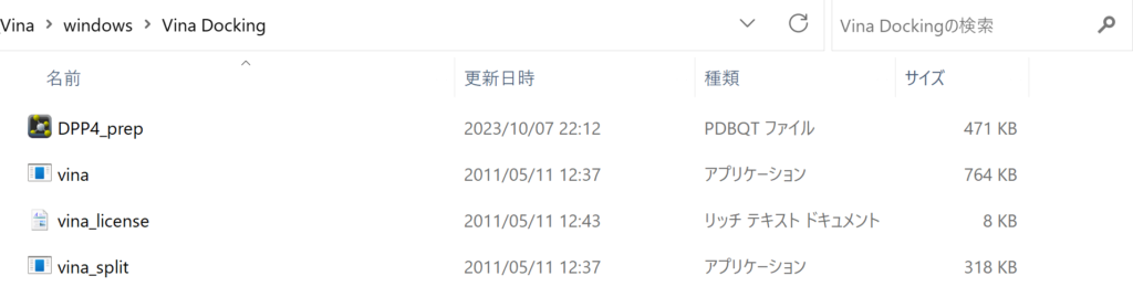
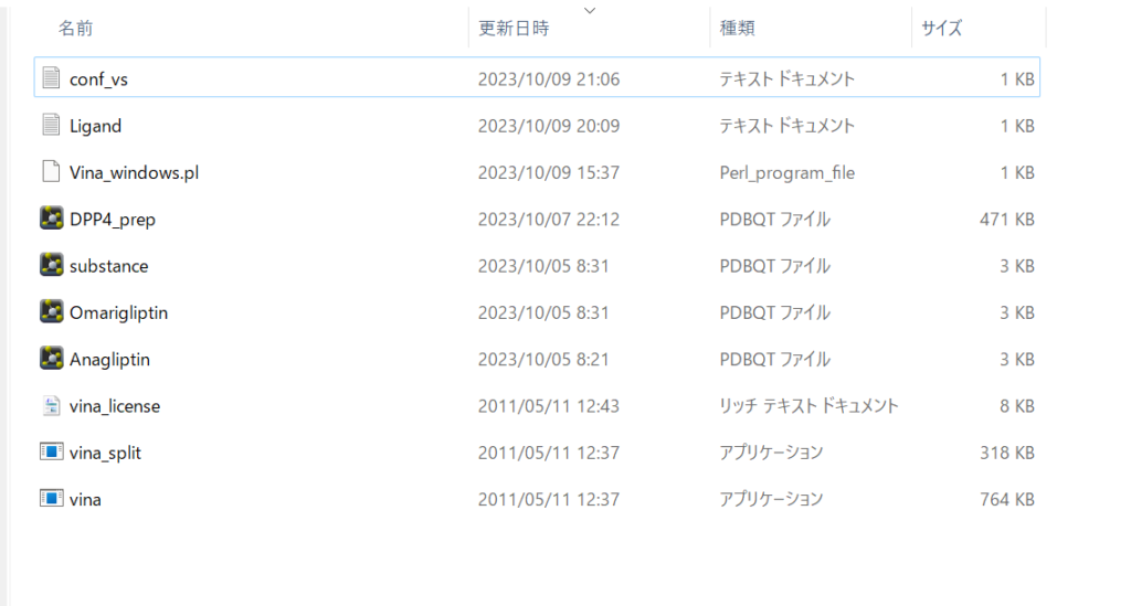
For in silico screening setup, first download AutoDock vina. Move the files vina, vina_license, and vina_split found in the downloaded AutoDock Vina folder (likely located in C:\Program Files (x86)\The Scripps Research Institute\Vina) to the directory containing your protein files. This directory is referred to as “Vina Docking” here.

Next, include the perl file in the same directory. Also, make sure all ligand files are placed in this directory.

Create a new text file named conf_vs.txt and insert the following content. Be cautious that the receptor file must have the .pdbqt extension to work properly:

receotor = DPP4_prep.pdbqt 

center_x = 18.171
center_y = 58.177 
center_z = 17.705

size_x = 80
size_y = 80
size_z = 80

num_modes = 10
energy_range = 4

The conf_vs.txt file serves as a configuration file for running docking calculations with AutoDock Vina. Here is an explanation of each item in the provided file:

receptor: Specifies the file name of the receptor used for docking. The receptor refers to the protein or other large molecule to which the ligand will bind. The .pdbqt format is a special format used by AutoDock and AutoDock Vina, containing information about atomic coordinates, atom types, and partial charges.
center_x, center_y, center_z: These specify the coordinates of the center of the search space, indicating the area where the ligand will attempt to bind to the protein. These coordinates are typically set to the center of the area of interest or a known binding site.
size_x, size_y, size_z: These specify the size of the search space in each direction (X, Y, Z) in Angstrom units, based on the size of the area you want to explore. Although 126 is the maximum, due to memory considerations, each dimension is set to 80.
num_modes: Indicates the maximum number of binding modes (binding structures) to be generated. AutoDock Vina can produce multiple different binding structures for a ligand, allowing the assessment of how a ligand might bind to the protein.
energy_range: Indicates the maximum energy difference between the best binding mode (lowest energy) and the worst binding mode to be displayed. A larger value may result in energetically unfavorable binding modes being displayed as well.

Using this configuration file to run AutoDock Vina will perform docking calculations based on the above settings.

Also, create a Ligand.txt file, which can be empty for now.

Your working directory should now look something like this.

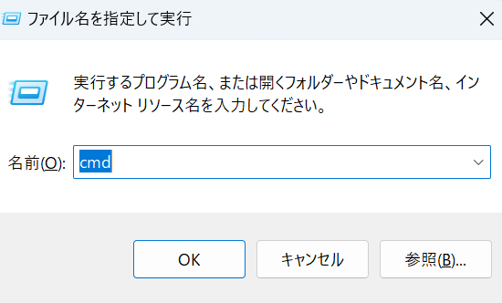
Next, open Command Prompt by pressing Windows+R, typing cmd, and launching it.

Download Perl from the provided link, specifically the dwimperl-5.14.2.1-v7-32bit.exe, and open Perl (Command line).

Execute the following code in Perl (command line):

dir /B > Ligand.txt

This command, used in the Windows Command Prompt, outputs only the names of files and subdirectories in the current directory to Ligand.txt.

Specifically:

dir: Command to display the contents of a directory.
/B: An option that displays only the names. Normally, the dir command shows details such as file size, creation date, and last modification date, but the /B option displays only the names.
>: Redirects the output. Specifying a file name after this symbol saves the command’s output to that file.
Ligand.txt: The name of the file where the output is saved.

Executing this command creates a file named Ligand.txt in the current directory, saving a list of names of files and subdirectories in the directory.

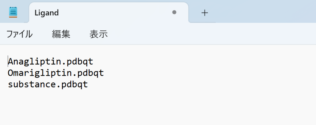
Upon opening the Ligand file, it should list the names of all files in the current directory. Delete everything except the ligand pdbqt files. For this screening, the file should list the following three ligands:

Anagliptin.pdbqt
Omarigliptin.pdbqt
substance.pdbqt

With this, the preparation for in silico screening is complete.

Conducting in silico screening

Now that we’ve completed the in silico screening preparation, let’s proceed with the actual screening process.

Execute the following command:

perl Vina_windows.pl

When prompted for the Ligand file, enter Ligand.txt and press Enter.

A screen similar to the one below will indicate that the screening is underway.

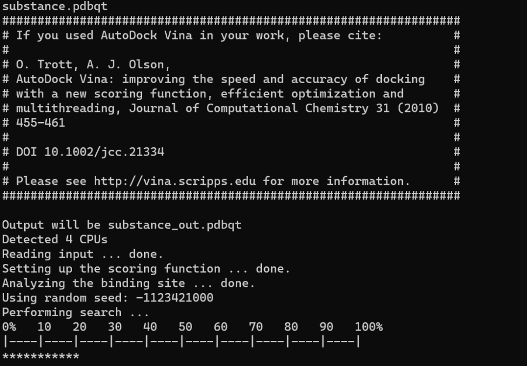
Once the calculation is complete, files named ligand_name_log and ligand_name_out will be generated for each ligand.

Results

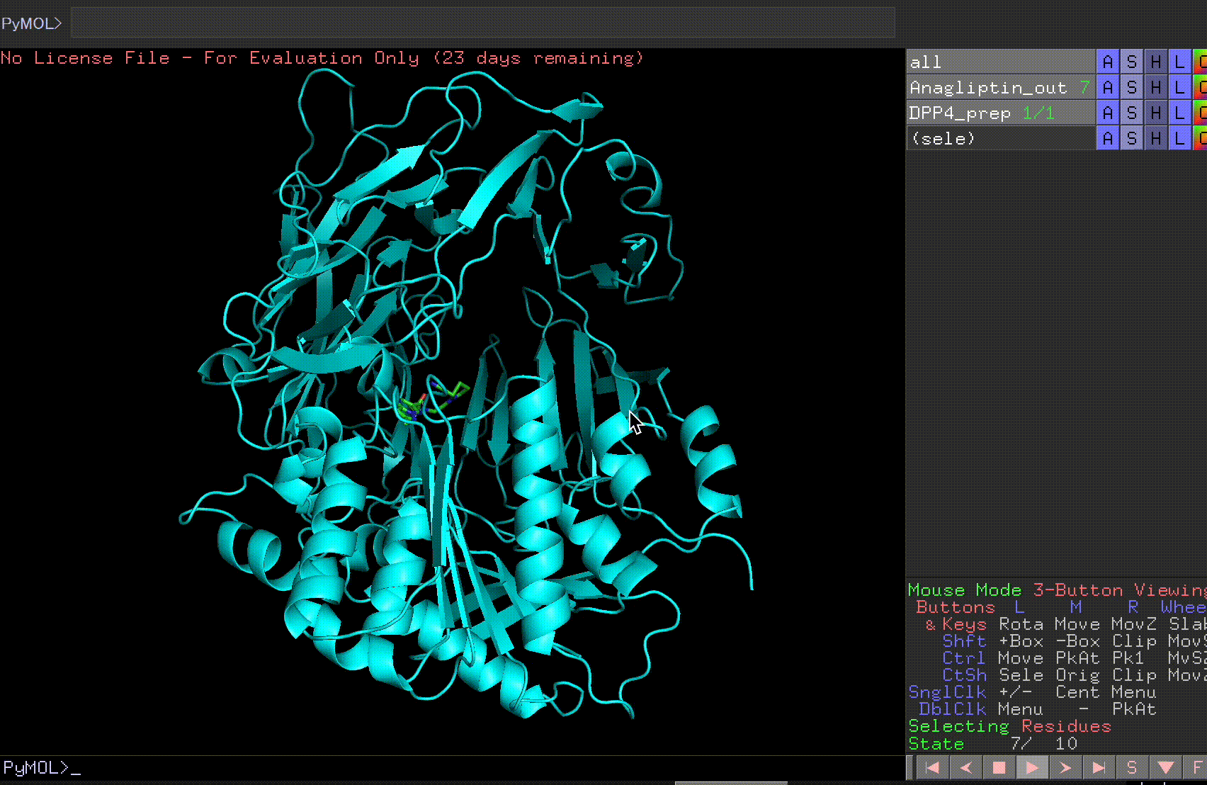
Let’s open the Anagliptin_out file and the DPP4_prep file.

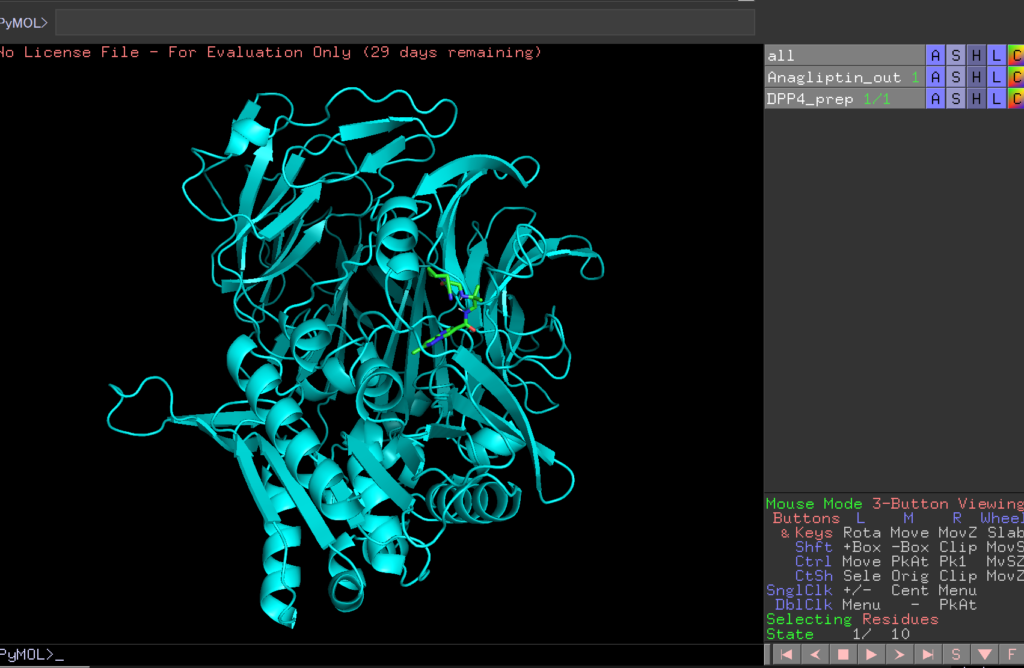
By pressing the play button in the bottom right corner, you can view the 10 predicted binding sites.

Review the Anagliptin.pdbqt_log to examine the binding affinity for each site. The highest binding affinity appears to be -6.9 kcal/mol.

mode |   affinity | dist from best mode
     | (kcal/mol) | rmsd l.b.| rmsd u.b.
-----+------------+----------+----------
   1         -6.9      0.000      0.000
   2         -6.7      3.102      4.347
   3         -6.6     20.983     24.994
   4         -6.6     34.775     36.825
   5         -6.6     37.303     39.078
   6         -6.6     33.968     36.318
   7         -6.5     27.023     28.704
   8         -6.5      3.644      5.007
   9         -6.4     54.846     57.680
  10         -6.4     27.367     28.847

The log displays the docking results of the ligand with the target protein by AutoDock Vina, showing multiple docking poses (modes) of the ligand, with the information listed for each pose:

mode: Number indicating the docking pose. Mode 1 is the most energetically favorable (most preferred) pose, followed by mode 2, and so on.
affinity (kcal/mol): Energy value indicating the binding affinity of this pose. Lower values indicate stronger binding between the ligand and the target protein.
dist from best mode: Distance based on comparison to the most preferred pose (mode 1).
rmsd l.b. (lower bound) and rmsd u.b. (upper bound): RMSD values indicating the average deviation of the ligand’s pose.

RMSD (Root Mean Square Deviation) values show the average deviation between the positions of atoms in two 3D structures; smaller values indicate more similarity between the structures. Larger RMSD values suggest significant differences between the structures.

Interpreting this log, the most preferred binding pose (mode 1) has a binding affinity of -6.9 kcal/mol, with subsequent poses showing slight variations in shape or position. Modes 2 and 8 are not far from mode 1, but modes 3 and onwards likely differ significantly from mode 1.

Let’s examine the binding sites for each ligand.

Also, open Omarigliptin_out and substance_out in PyMOL.

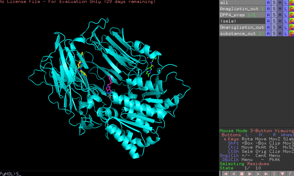
In the image below, green represents Anagliptin_out, red is Omarigliptin_out, and yellow is substance_out.

The binding affinities for each ligand are as follows:

Anagliptin_out
mode |   affinity | dist from best mode
     | (kcal/mol) | rmsd l.b.| rmsd u.b.
-----+------------+----------+----------
   1         -6.9      0.000      0.000
   2         -6.7      3.102      4.347
   3         -6.6     20.983     24.994
   4         -6.6     34.775     36.825
   5         -6.6     37.303     39.078
   6         -6.6     33.968     36.318
   7         -6.5     27.023     28.704
   8         -6.5      3.644      5.007
   9         -6.4     54.846     57.680
  10         -6.4     27.367     28.847

Omarigliptin_out
mode |   affinity | dist from best mode
     | (kcal/mol) | rmsd l.b.| rmsd u.b.
-----+------------+----------+----------
   1         -8.2      0.000      0.000
   2         -7.5      4.813      9.825
   3         -7.0      1.396      2.552
   4         -7.0     22.600     25.155
   5         -6.9     26.790     28.270
   6         -6.8     24.370     25.515
   7         -6.8      5.341      8.885
   8         -6.7     35.981     37.517
   9         -6.7     23.764     25.377
  10         -6.7     20.055     22.510

substance_out
mode |   affinity | dist from best mode
     | (kcal/mol) | rmsd l.b.| rmsd u.b.
-----+------------+----------+----------
   1         -8.1      0.000      0.000
   2         -7.9     25.160     28.365
   3         -7.9     35.292     37.012
   4         -7.9     29.785     33.301
   5         -7.8     38.196     39.991
   6         -7.8     26.114     28.770
   7         -7.7     49.792     53.366
   8         -7.7     23.544     28.206
   9         -7.7     24.302     27.489
  10         -7.7      3.062      6.948

Here’s how to interpret this data:

Binding Affinity: Comparing the binding affinity (affinity) of the most favorable binding poses for all ligands, Omarigliptin exhibits the highest affinity, followed by the substance, and finally Anagliptin. This metric indicates how strongly each ligand binds to the target protein.
Diversity of Docking Poses: The RMSD values represent the deviation of other poses from the most favorable one. Poses with low RMSD values are structurally similar to the most favorable pose, indicating similar binding modes or positions. Conversely, high RMSD values suggest different binding modes or positions, indicating a variety of ways the ligand might interact with the target protein.
Reliability of Results: When the range of RMSD (between l.b. and u.b.) is narrow, the results for that pose are considered relatively reliable. A wide RMSD range, on the other hand, indicates uncertainty in the accuracy of that pose’s prediction. This can be useful in assessing the confidence level in each predicted binding mode’s relevance and stability.

For Anagliptin, the second and eighth poses are relatively close to the most favorable one, but other poses might significantly differ. This suggests that while Anagliptin has a preferred binding mode, it can also adopt several other substantially different configurations when interacting with the target.

In the case of Omarigliptin, the first three poses are similar, indicating a higher consistency in how this molecule interacts with the target protein. This consistency might imply a more predictable and reliable interaction pattern, which could be advantageous in a therapeutic context.

For the substance, the first and tenth poses are relatively close, which is an unexpected result, especially since this substance was chosen randomly. It’s surprising that a randomly selected substance shows higher binding affinity than a known drug like Anagliptin. However, the fact that the most potent binding mode of the substance (mode 1) is less frequent among other modes suggests that while the substance can achieve a high binding affinity, it might not do so as consistently as Omarigliptin. This could mean that, despite the high affinity in the best-case scenario, the substance might not be as reliable a binder as Omarigliptin, which shows high affinity across multiple modes.

This analysis highlights the importance of not only considering the highest binding affinity when evaluating potential drug candidates but also considering the diversity and consistency of binding modes. A compound like Omarigliptin, with consistently high affinity across several modes, might be more desirable than a compound like the substance, which has a high affinity but less consistency and predictability in its binding behavior.

Finally…

The PyRx I previously introduced is a tool that makes screening with Autodock Vina more accessible. If you found today’s operations a bit challenging, using PyRx could be a good alternative, especially for beginners!

As demonstrated, in silico screening can be conducted easily on a computer. I encourage you to try it out and experience drug discovery for yourself!