![Numerical Solutions to Hyperbolic Partial Differential Equations with Code [Python]](https://labo-code.com/wp-content/uploads/2024/02/Hyperbolic-Partial-Differential-Equation.png)
In this article, we will delve into the numerical solutions of hyperbolic partial differential equations, with easy-to-understand concrete examples. We will learn an approach using Python.
Through this article, let’s master one of the numerical solutions for partial differential equations!
Note: The discussion is limited to the finite difference method. Details on errors and boundary conditions are omitted to avoid redundancy.
macOS Monterey(12.7.1), python3.11.4
What is Numerical Solution of Partial Differential Equations?
The numerical solution of partial differential equations (PDEs) refers to methods used to approximate the solutions of PDEs. Since analytical solutions are often not possible, numerical methods become necessary. Below, we introduce several main numerical methods.
1. Finite Difference Method: This method discretizes space and time into a grid and approximates derivatives with differences. While intuitive and relatively easy to implement, the choice of grid significantly affects the solution’s accuracy.
2. Finite Element Method: The problem domain is divided into small “elements,” and equations are approximated within each element. This method is suitable for problems with complex shapes or boundary conditions.
3. Finite Volume Method: Particularly suited for conservation law equations, the domain is divided into small “volumes,” and average values within each volume are calculated.
4. Spectral Method: The equation is represented as a sum of waves with different frequencies, and solving involves calculating the coefficients of these waveforms. High accuracy can be achieved, but smooth solutions are required.
5. Finite-Difference Time-Domain (FDTD) Method: A type of finite difference method used extensively in electromagnetics, applied in the time domain.
These methods are used in physics, engineering, meteorology, and other fields to solve PDEs. Each method has its characteristics and applicable problem types, so choosing the optimal method according to the problem’s nature is necessary. In advanced computer simulations, these methods are often combined.
This article introduces the Finite Difference Method for numerical solutions.
Difference Approximation
In the numerical solution of partial differential equations, the finite difference method is very commonly used.
The finite difference method utilizes difference approximations. The details of the concept of difference approximation for partial derivatives are covered in another article, and here we will briefly introduce only the difference approximation used for parabolic equations, which is the main topic of this article.
Let $u = u(x,y)$ be given in the domain $0 \leqq x \leqq a, 0 \leqq y \leqq b$. Divide this domain into a grid (difference grid) as shown below. The grid spacing can be equal or, as shown in the figure, unequal.
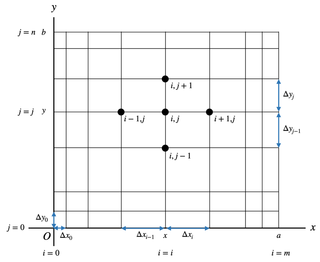
Label the grid points in the $x$ direction as $i=0 \sim m$ and in the $y$ direction as $j=0 \sim n$. Label the point $(x,y)$ on the grid as $(i,j)$ and the value of $u$ at this point as $u_{i,j}$. Label the neighboring grid points as shown in the figure with $\Delta x_i,\Delta y_i$, etc. The difference approximations for partial derivatives $∂u/∂x, ∂u/∂y$ can be represented as follows, fixing $j$ for $∂u/∂x$ and $i$ for $∂u/∂y$.
When the grid spacing is uniform,
$$
\begin{aligned}
\Delta x_{i-1} &= \Delta x_{i} =h \\
\Delta y_{i-1} &= \Delta y_{i} =k \end{aligned}
$$
thus, the first-order partial derivative coefficients are obtained using the forward difference approximation as follows:
$$
\begin{aligned}
\frac{∂u}{∂x} &= \frac{1}{h}(u_{i+1,j} – u_{i,j}) \\
\frac{∂u}{∂y} &= \frac{1}{k}(u_{i,j+1} – u_{i,j})
\end{aligned}
$$
Furthermore, the second-order partial derivative coefficients are obtained using the central difference approximation as follows:
$$
\begin{align*}
\frac{∂^2u}{∂x∂y} &= \frac{1}{4hk}(u_{i+1,j+1} – u_{i+1,j-1} – u_{i-1,j+1} + u_{i-1,j-1}) \\
\frac{∂^2u}{∂x^2} &= \frac{1}{h^2}(u_{i+1,j} – 2u_{i,j} + u_{i-1,j}) \\
\frac{∂^2u}{∂y^2} &= \frac{1}{k^2}(u_{i,j+1} – 2u_{i,j} + u_{i,j-1})
\end{align*}
$$
These difference approximations are used to convert partial differential equations into difference equations.
Overview of Numerical Solution using the Finite Difference Method
The steps for numerically solving a partial differential equation using the finite difference method are:
1. Convert the partial differential equation into a difference equation.
2. Calculate the values of each element using the difference equation.
Let’s explain each step below.
Converting Partial Differential Equations to Difference Equations
Hyperbolic Equation
$$
\frac{∂^2u}{∂t^2} = p(x,t) \frac{∂^2u}{∂x^2} + q(x,t); \ \ \ \ \ \ 0 \leqq x \leqq a, 0 \leqq t < \infty \ \ \ \ (1)
$$
Where in the given domain $p(x,t) > 0$. Let’s consider solving this equation under the following conditions: (Assuming $p(x,t), q(x,t), a, f_1(x), f_2(x), g_1(t), g_2(t)$ are known)
Initial conditions: $u(x,0)= f_1(x), \ \ ∂u/∂t |_{t=0} \equiv \frac{∂u(x,0)}{∂t} = f_2(x)$
Boundary conditions: $u(0,t) = g_1(t), \ \ \ u(a,t) = g_2(t)$
First, we will express equation $(1)$ as a difference equation using the difference approximations for partial derivatives discussed in the previous section, namely
$$
\frac{(u_{i,j+1} – 2u_{i,j} + u_{i,j-1}) }{k^2} = p_{i,j} \frac{(u_{i+1,j} – 2u_{i,j} + u_{i-1,j}) }{h^2} + q_{i,j}
$$
By rearranging this equation, we get
$$
\begin{align*} u_{i,j+1} &= R (u_{i+1,j} + u_{i-1,j}) + S u_{i,j} – u_{i,j-1} + Q \ \ \ \ (2) \\ R &= \frac{k^2}{h^2}p_{i,j}, \ \ S=2(1-R), \ \ Q=k^2q_{i,j} \end{align*}
$$
Calculating the Values of Each Element Using Difference Equations
Let’s take a closer look at difference equation $(2)$.
For example, if we want to find $u_{i,1}$, by substituting $j=0$ into equation $(2)$, we get
$$
u_{i,1} = R (u_{i+1,0} + u_{i-1,0}) + S u_{i,0} – u_{i,-1} + Q \ \ \ \ (3)
$$
You might have noticed the appearance of $u_{i,-1}$, a negative grid point which doesn’t actually exist. Hence, we consider it a virtual grid point.
This virtual grid can be replaced using the initial condition $∂u/∂t |_{t=0} \equiv \frac{∂u(x,0)}{∂t} = f_2(x)$.
Expressing $∂u/∂t = f_2(ih)$ in terms of difference equations gives us
$$
\frac{u_{i,j+1} – u_{i,j-1}}{2k} = f_2(ih)
$$
$$
u_{i,j-1} = -2kf_2(ih) + u_{i,j+1}
$$
Substituting $j=0$ into this, we find
$$
u_{i,-1} = u_{i,1} – 2kf_2(ih)
$$
Inserting this into equation $(3)$ gives
$$
u_{i,1} = R (u_{i+1,0} + u_{i-1,0}) + S u_{i,0} – u_{i,1} + 2kf_2(ih) + Q
$$
$$
u_{i,1} = \frac{1}{2} ( R (u_{i+1,0} + u_{i-1,0}) + S u_{i,0} + 2kf_2(ih) + Q )
$$
By doing so, the value of $u_{i,1}$ can be determined by the initial and boundary conditions.
Example Problem
Please solve the following partial differential equation under the given conditions.
$$
\frac{\partial^2 u}{\partial t^2} = (x + 1) \frac{\partial^2 u}{\partial x^2} + x e^{-t}; 0 \leqq x \leqq 1, 0 \leqq t < \infty
$$
Initial conditions: $u(x,0) = \sin \pi x, \frac{\partial u (x,0)}{\partial t} = 0$
Boundary conditions: $u(0, t) = 0, u(1, t) = 0$
Let’s denote the grid numbers as $i=0 \sim m, j=0 \sim n$, and the value of $u$ at any grid point as $u_{i,j}$.
As introduced above, the first step is to convert this partial differential equation into a difference equation, and then implement a program to solve the difference equation.
Implementation Method
The code can be implemented as follows:
The creation of graphs and output to text files is also included, making the code somewhat lengthy, but the crucial part is the calculate_equation function.
Save the following implementation as main.py in a folder (here, ~/Desktop/labcode/python/numerical_calculation/hyperbolic_equation).
import matplotlib.pyplot as plt
from matplotlib.animation import ArtistAnimation
import numpy as np

def _set_initial_condition(
    *,
    array_2d: list,
    grid_counts_x: int,
    grid_space: float,
) -> None:
    """
    Set initial conditions

    Sets the U value at t=0 for all but the boundary points
    """
    for i in range(1, grid_counts_x):
        array_2d[i][0] = np.sin(np.pi * i * grid_space)

def _set_boundary_condition(
    *,
    array_2d: list,
    grid_counts_x: int,
    grid_counts_t: int,
) -> None:
    """Set boundary conditions"""
    for j in range(grid_counts_t + 1):
        array_2d[0][j] = 0.0
        array_2d[grid_counts_x][j] = 0.0

def calculate_equation(*, M: int, N: int, H: float, K: float) -> list:
    """
    Calculate the difference equation

    The core function of this program
    """
    # List for U values
    U: list = [[0.0 for _ in range(N + 1)] for _ in range(M + 1)]

    # Setting initial conditions
    _set_initial_condition(
        array_2d=U,
        grid_counts_x=M,
        grid_space=H,
    )
    # Setting boundary conditions
    _set_boundary_condition(
        array_2d=U,
        grid_counts_x=M,
        grid_counts_t=N,
    )

    # Calculating U[i][1]
    for i in range(1, M):
        R = (K / H) ** 2 * (i * H + 1)
        S = 2 * (1.0 - R)
        Q = K**2 * i * H * np.exp(0)
        U[i][1] = (R * (U[i + 1][0] + U[i - 1][0]) + S * U[i][0] + Q) / 2.0

    # Calculating U[i][j + 1]
    for j in range(1, N):
        for i in range(1, M):
            R = (K / H) ** 2 * (i * H + 1)
            S = 2 * (1.0 - R)
            Q = K**2 * i * H * np.exp(-j * K)
            U[i][j + 1] = (
                R * (U[i + 1][j] + U[i - 1][j]) + S * U[i][j] - U[i][j - 1] + Q
            )

    return U

def animate_time_evolution(
    *,
    array_2d: list,
    grid_counts_x: int,
    grid_counts_t: int,
    grid_space: float,
    time_delta: float,
) -> None:
    """
    Create an animation of the dot-line plot
    Plot the data in array_1d and show the time evolution in an animation
    """
    # Transpose 2D array
    array_2d = np.array(array_2d).T
    # Generate values for the x-axis
    x_values = np.arange(grid_counts_x + 1) * grid_space

    # Creating the animation
    path_gif = "./animation.gif"
    frames = []

    fig, ax = plt.subplots(figsize=(7, 5))
    plt.xlabel("X (m)")
    plt.ylabel("Temperature (deg.)")
    plt.grid(True)

    for j in range(grid_counts_t + 1):
        frame = plt.plot(
            x_values,
            array_2d[j],
            linestyle="--",
            marker="o",
            color="b",
        )

        time = j * time_delta
        text = ax.text(
            0.05,
            0.95,
            f"t = {time:.2f} (h)",
            transform=ax.transAxes,
            fontsize=14,
            verticalalignment="top",
        )
        frames.append(frame + [text])

    anim = ArtistAnimation(fig, frames, interval=100)
    anim.save(path_gif, writer="pillow")

def output_result_file(
    array_2d: list,
    grid_counts_x: int,
    grid_counts_t: int,
    grid_space: float,
    time_delta: float,
) -> None:
    """Write a 2D array to a text file"""
    with open("./calculated_result.txt", "w") as file:
        file.write(f"# This file shows calculated result as below.\n\n")
        file.write(f"# Calculation Parameters.\n")
        file.write(f"grid_counts_x: {grid_counts_x}\n")
        file.write(f"grid_counts_t: {grid_counts_t}\n")
        file.write(f"grid_space: {grid_space}\n")
        file.write(f"time_delta: {time_delta}\n\n")

        file.write(f"# Calculated Matrix U.\n")
        for row in array_2d:
            line = " ".join(map(str, row))
            file.write(line + "\n")

def validate_parameters(R: float) -> None:
    """Check the validity of parameters"""
    if R > 1.0:
        raise ValueError("R must be less than 1.0.")

if __name__ == "__main__":
    """
    Numerical solution of hyperbolic equations (explicit method)
    """
    grid_counts_x: int = 10  # Value of grid point number m
    grid_counts_t: int = 40  # Value of grid point number n
    grid_space: float = 0.1  # Step size (meter)
    time_delta: float = 0.05  # Step size (hour)

    validate_parameters(R=2 * (time_delta / grid_space))

    array_2d = calculate_equation(
        M=grid_counts_x,
        N=grid_counts_t,
        H=grid_space,
        K=time_delta,
    )
    animate_time_evolution(
        array_2d=array_2d,
        grid_counts_x=grid_counts_x,
        grid_counts_t=grid_counts_t,
        grid_space=grid_space,
        time_delta=time_delta,
    )
    output_result_file(
        array_2d=array_2d,
        grid_counts_x=grid_counts_x,
        grid_counts_t=grid_counts_t,
        grid_space=grid_space,
        time_delta=time_delta,
    )
Executing the Program
Open the terminal and enter:
$ cd Desktop/labcode/python/numerical_calculation/hyperbolic_equationThen, execute the following command (ignore the $ symbol):
$ python main.pyExecution Results
If a file named animation.gif has been created in ~/Desktop/LabCode/python/numerical_calculation/hyperbolic_equation and it turns into a gif image like the following, then it’s a success!
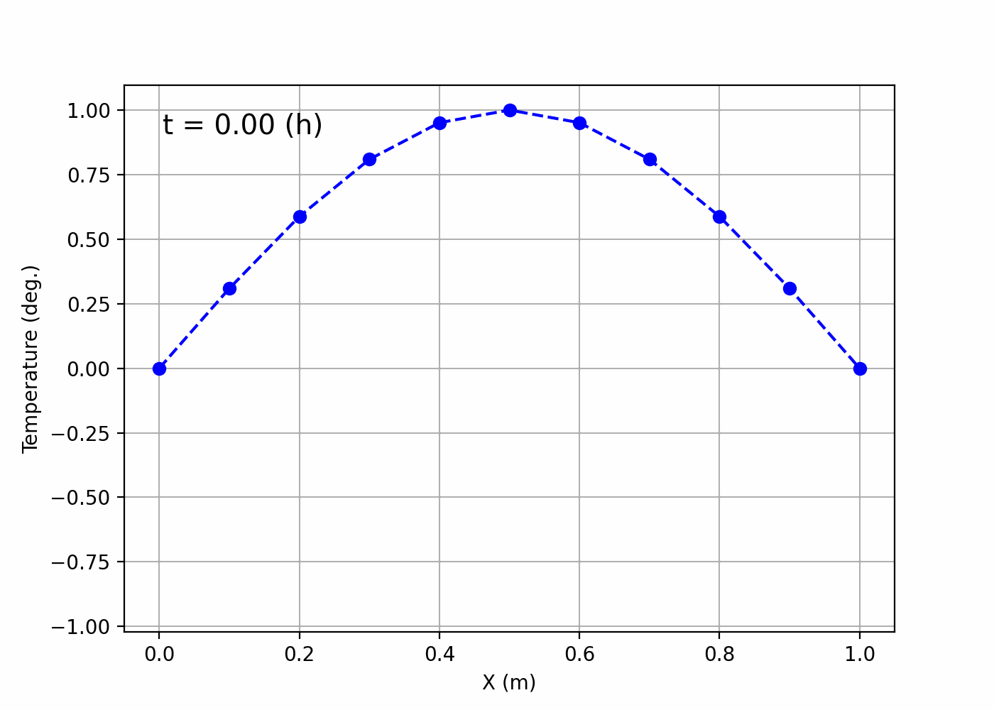
It seems like the situation where a string is swinging up and down has been visualized.
Additionally, a text file named calculated_result.txt should have been created as follows. Although only basic information is outputted this time, by outputting the calculation results along with the parameters used for the calculation, it becomes possible for others to evaluate the results. For your own benefit as well as for the benefit of others, make it a habit to output the results.
# This file shows calculated result as below.

# Calculation Parameters.
grid_counts_x: 10
grid_counts_t: 40
grid_space: 0.1
time_delta: 0.05

# Calculated Matrix U.
0.0 0.0 0.0 0.0 0.0 0.0 0.0 0.0 0.0 0.0 0.0 0.0 0.0 0.0 0.0 0.0 0.0 0.0 0.0 0.0 0.0 0.0 0.0 0.0 0.0 0.0 0.0 0.0 0.0 0.0 0.0 0.0 0.0 0.0 0.0 0.0 0.0 0.0 0.0 0.0 0.0
0.3090169943749474 0.3049827931120519 0.2927821760958873 0.2722125088561874 0.24313249125986083 0.2056500846551192 0.16025988763305207 0.10790150134761026 0.049957056241041804 -0.011776227735267425 -0.07511760786572898 -0.13754506237975533 -0.19627228588447948 -0.2483850607628004 -0.2910494490618322 -0.3217810901327259 -0.33872980098363337 -0.34090019579050934 -0.32823116914706624 -0.30151830303315574 -0.26225260404213835 -0.21248646260817422 -0.15477070801737391 -0.09208545147202046 -0.02763894080408742 0.0354929092367792 0.09474601028741463 0.14825999445084737 0.19479726271990142 0.23351002385827413 0.2637698944599734 0.28516869573600334 0.2976070799025527 0.3013022383634498 0.29663949096085396 0.28395511520066646 0.26340675931670643 0.2350142105333222 0.19882915277839425 0.1551334956238426 0.10459537550306455
0.5877852522924731 0.5794047749172154 0.5543088628170679 0.5126958273460732 0.45496653998632314 0.38183656708080815 0.2945074341077582 0.19484943599137944 0.08552713473208474 -0.029979739805290357 -0.14746324136234149 -0.26215923909875755 -0.3689909509784872 -0.46288693921615043 -0.5391585312066091 -0.5938718581498124 -0.6241287517745315 -0.6282274180634483 -0.605763439910379 -0.5577415238072453 -0.4866562168746265 -0.396383366236136 -0.2917731099124619 -0.17805419410682333 -0.060332278626518375 0.05662081778466293 0.16837474844587952 0.27091443995791226 0.36091759317919675 0.43606901823037764 0.4951148730446506 0.5375611038249619 0.5632370694954658 0.5720375009427245 0.5639433483267814 0.5391559627299322 0.49813890910075964 0.4415490819280186 0.3702110635406817 0.2852559676690559 0.188369752755483
0.8090169943749473 0.7965232585985789 0.7592704092720312 0.6980237929127329 0.6141004189717728 0.5093945146429286 0.38642406640356547 0.24840854667589776 0.09936476888613366 -0.055834722193602956 -0.21152807988969136 -0.3615207126461062 -0.49950522332576336 -0.6195109064734203 -0.7162343720335208 -0.7852284593598534 -0.8230824930529504 -0.8277248504163482 -0.7987802002730451 -0.7377313435221419 -0.647714483089495 -0.5330721471620046 -0.398968098673832 -0.2512073324417034 -0.09609033703254855 0.05994066583789725 0.21083513645200833 0.3513483573947398 0.4771211681315775 0.5845518279992986 0.6707558879158749 0.7336988815915186 0.7722787841475706 0.7861374001302917 0.7752986232162671 0.7399682935790364 0.6806863155925486 0.5986612539968726 0.4959534349899685 0.3753709194551349 0.24025537802143512
0.9510565162951535 0.9352647096074655 0.8883168938922941 0.8115908705902218 0.707398671948937 0.5789566329809795 0.43033859053378526 0.2664083523469224 0.09271485434941559 -0.08468074375135591 -0.25945191243276705 -0.425265540904309 -0.5759665147347939 -0.705702002176888 -0.8091350151498963 -0.881859587589341 -0.9208833740033349 -0.9248639864377418 -0.8939530241348044 -0.8294813235011836 -0.7338510080306243 -0.6106862842452613 -0.464910581493102 -0.30245661969968485 -0.12973112835440392 0.04679463434042434 0.22072429825458287 0.38582891975040373 0.5363182858775802 0.6671807064844799 0.774309475522349 0.8543834990505005 0.9047890866094387 0.9238021290772088 0.910873696978843 0.8666822280993867 0.7928735443140164 0.6917713174935313 0.5663515818474197 0.42044054369488726 0.25883271358109905
1.0 0.9822711936106826 0.9296975356413092 0.8442239959373173 0.7290724361268137 0.5886478819981495 0.4283873604915754 0.25449973544548227 0.07357231081469656 -0.10785019025842718 -0.2835157176896811 -0.44747978393200727 -0.5940944497086907 -0.7182347301879992 -0.8157160718954938 -0.8835523744682285 -0.9198446977666628 -0.9235340944437193 -0.8943996517938706 -0.8333116640131276 -0.7423688790470901 -0.6246974464208462 -0.484151955862201 -0.32526335615056695 -0.1533745564258732 0.025412592621437396 0.2046203908818099 0.37781092316523823 0.5387338536686733 0.6813289510921626 0.7999262755006344 0.8896947338150822 0.9470295559022702 0.9696567880962499 0.9566038555838664 0.9082790516215525 0.8266069389688095 0.7149535352989325 0.5777758112030321 0.42025569355509024 0.2481638741071843
0.9510565162951536 0.9331873086520817 0.8803290347045547 0.7948467077456308 0.6806224462793355 0.5428472153973213 0.3876277936083759 0.2214693593524663 0.05087516328029061 -0.1177931342259182 -0.27839739530849683 -0.4253521250859268 -0.5541200626765675 -0.6614171073968096 -0.7448989752943701 -0.8027024384581181 -0.8333626470867074 -0.8360986806844454 -0.8109920579696874 -0.7588183487758012 -0.6808366211069099 -0.5788775799403985 -0.45558794276899 -0.3144583484645533 -0.15962636701007166 0.004197266147748216 0.17156200159373927 0.3362151876312711 0.491453210033439 0.6307012333661528 0.7479223320276944 0.8378087787275489 0.8960434637532305 0.9197241748695867 0.9076667452422327 0.8603704721577393 0.7798392279505066 0.669546774747226 0.5344550956891249 0.3807387250434341 0.21515931268026817
0.8090169943749475 0.7930636475904655 0.746007260921673 0.6703869283739219 0.5702247925685181 0.45051556859264735 0.3167426272302094 0.17470699838233988 0.030479061988168264 -0.10996709270291546 -0.24142973463836326 -0.3599210475618002 -0.4625264871037999 -0.54701921421177 -0.6117480617479326 -0.6557657406828898 -0.6787551424450636 -0.6806594321387394 -0.6614413841717108 -0.6212552661889166 -0.560740627327072 -0.481043490006875 -0.3836723034070762 -0.27058476078859867 -0.14452852663059523 -0.009239697593738739 0.13070274456064307 0.27010939203147183 0.40327283010978837 0.5241265653818611 0.62674502054998 0.7059974895527332 0.7579153248883971 0.7797260226263198 0.7699474630425529 0.7287228125991388 0.6580486236112529 0.5615523101847922 0.4440117688841584 0.31103062446964036 0.16885394055860917
0.5877852522924732 0.5758395362295867 0.5407504015846227 0.48463763790480924 0.41046274594392795 0.3218859953010506 0.2233654152717499 0.11988460987501386 0.016221129219635394 -0.0836289017909767 -0.17643877900937394 -0.2594871201240938 -0.33057457724664435 -0.38826767523267 -0.4319097498025059 -0.4612957824241638 -0.4763857874944956 -0.47728050940528305 -0.4642281854061583 -0.4374528328067261 -0.39702414075593423 -0.3430643219118048 -0.27614764846349893 -0.19750040324649684 -0.10894714505580902 -0.01290670904576693 0.08746060441845853 0.1882462320819253 0.28511304431992207 0.373679478319645 0.4496701468472645 0.5089954530337145 0.5481155236606657 0.5646094123553451 0.5574851525446628 0.527066581404044 0.47481943693561685 0.4033945681747775 0.31662174043795954 0.2191001259622241 0.11558358779491351
0.3090169943749475 0.30295791946630984 0.28475286697885804 0.2549249158047677 0.21505776556788883 0.16769768655930678 0.11567295484929299 0.06152432928306593 0.007458328790424913 -0.044479827570212765 -0.09245121274871328 -0.13503767186103538 -0.17129658769096237 -0.20061184322541958 -0.22259839043353413 -0.2371562809524509 -0.24446837647434985 -0.2448077732362381 -0.23832634379432496 -0.22502849408131198 -0.20487350327147494 -0.17784742247016966 -0.14403448329481042 -0.10380995807122258 -0.058066231490956396 -0.00823179191898847 0.04393679897221464 0.09652241447290816 0.1474119870497067 0.19424371115011552 0.234569445007957 0.2661495687210239 0.28713800028124264 0.2961544724785851 0.29244577898445734 0.2761300808429286 0.24823842344030217 0.21043141881230523 0.16468076981984328 0.11321524559981189 0.05858791455308532
0.0 0.0 0.0 0.0 0.0 0.0 0.0 0.0 0.0 0.0 0.0 0.0 0.0 0.0 0.0 0.0 0.0 0.0 0.0 0.0 0.0 0.0 0.0 0.0 0.0 0.0 0.0 0.0 0.0 0.0 0.0 0.0 0.0 0.0 0.0 0.0 0.0 0.0 0.0 0.0 0.0
In Conclusion
We have introduced the numerical solution of hyperbolic partial differential equations using the finite difference method.
The Python computation program is also generously shared, so please deepen your understanding by running it.
In the future, we will write new articles on numerically solving other types of partial differential equations, so we hope you will look forward to them.