【scRNA-seq】Assigning cell types to each cluster automatically using Seurat in single-cell RNA sequencing【bioinformatics】

In our previous session, we explained how to create a Seurat object and perform cell clustering using Seurat in a hands-on manner.

In this article, we will delve deeper into the use of Seurat by attempting to label each cluster with cell types based on biomarkers.

By utilizing the SingleR library, it is possible to automatically assign cell types, eliminating bias. I encourage you to give it a try.

Tested Environment

macOS Monterey (12.4), Quad-Core Intel Core i7, Memory 32GB

Beginner-Friendly Technical Book on Single Cell RNA-seq Analysis Using Public Data Available for Sale

¥3,600 → ¥1,800 50%OFF!!

Easy-to-Understand Explanation for Programming Beginners!
Start Single Cell RNA-seq Analysis with R and Seurat!

Go To Technical Book Page

Objective of This Analysis

At the end of our last hands-on session, I believe we performed a UMAP plot and obtained the following output.

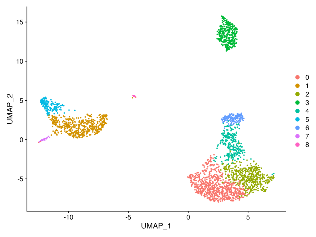
In the above, we were able to divide the data into 8 clusters. However, questions arise such as:

What cell type does each cluster represent?
Are there biomarkers that are specifically expressed in each cluster?

These questions can also be analyzed using Seurat.

Data Verification

Let’s proceed with the analysis. The dataset we will be using is as follows:

Paper Title: Immunophenotyping of COVID-19 and influenza highlights the role of type I interferons in development of severe COVID-19

Dataset：GSE149689

This paper utilizes Single Cell RNA-seq analysis to explore the role of type I interferon responses in the progression of severe COVID-19. The GSE149689 dataset used in this paper has been reanalyzed in the following publication:

Early peripheral blood MCEMP1 and HLA-DRA expression predicts COVID-19 prognosis

This publication reanalyzes seven datasets, including GSE149689, to examine the expression of MCEMP1 and HLA-DRA genes in CD14+ cells as prognostic biomarkers for severe COVID-19.

Thus, scRNA-seq data available in public databases can be reanalyzed and published as new papers.

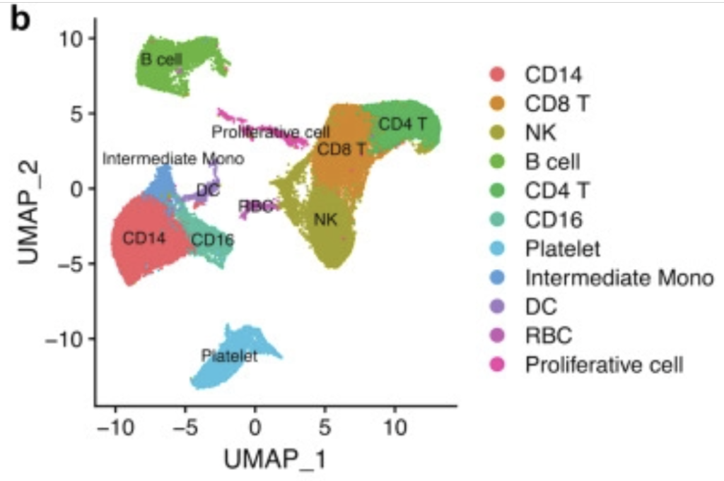
In this session, let’s attempt to replicate Fig4b from Early peripheral blood MCEMP1 and HLA-DRA expression predicts COVID-19 prognosis using the GSE149689 dataset with Seurat. While it may be challenging to create an exact replica, it is possible to produce a similar figure.

Basic Seurat Processing

We will download the GSE149689 dataset. Please access it from the link provided.

If you scroll to the bottom of the page, you should find the Supplementary file section. Please click either ftp or http and download all three files.

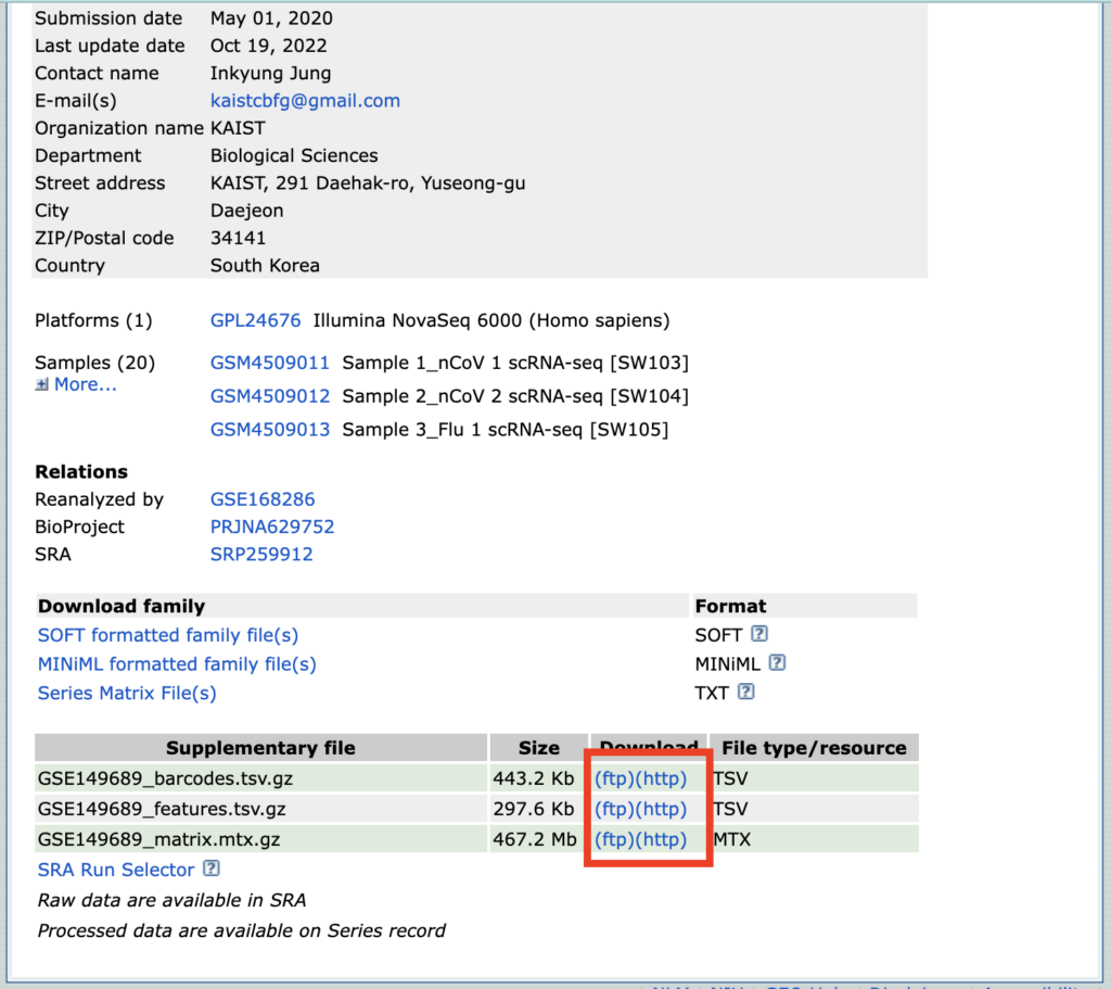
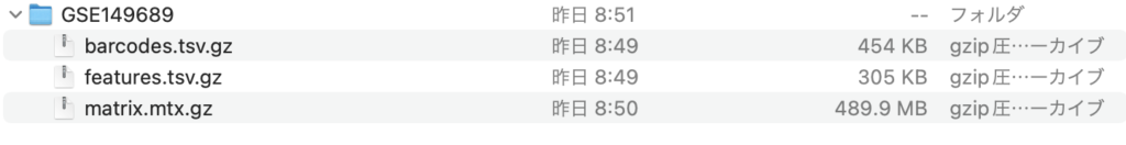
Once downloaded, please rename the files, leaving only the names as barcodes, features, and matrix, as shown below.

To launch RStudio and set the Working Directory.

This time, a folder named “GSE149689” has been created on the desktop, and the files downloaded earlier are stored in this folder, with the Desktop folder set as the Working Directory. There should be no issues as long as the path is correctly specified when loading the data later on.

Next, we will proceed to create a Seurat object. Please code the following in the editor.

install.packages("dplyr")
install.packages("Seurat")
install.packages("patchwork")
library(dplyr)
library(Seurat)
library(patchwork)

# Load the dataset
pbmc.data <- Read10X(data.dir = "./GSE149689/")

# Initialize the Seurat object with the raw (non-normalized data).
pbmc <- CreateSeuratObject(counts = pbmc.data, project = "pbmc3k", min.cells = 3, min.features = 200)

The explanations for each argument used in CreateSeuratObject are as follows, using mostly default values:

counts: A matrix containing gene expression data for each cell. In this example, pbmc.data is used as the input.
project: The name assigned to the created Seurat object. In this example, “PBMC” is specified.
min.cells: A threshold to include genes detected in at least this number of cells. In this example, genes detected in at least 3 cells are included.
min.features: A threshold to include cells that have detected at least this number of genes. In this example, cells with at least 200 detected genes are included.

Next, we will proceed with Quality Control (QC) and normalization. The conditions are written in the paper, so let’s look at the Materials and Methods section.

Single-cell data processing and analysis

Integrative analysis of single-cell data was performed using the Seurat R package (Version 3), and single-cell visualisation was performed using Uniform Manifold Approximation and Projection (UMAP). During quality control, cells with a mitochondrial gene ratio of more than 15% were removed, which may be potentially dead cells. Only those cells with gene numbers in the range of 200–5000 or RNA numbers detected between 1000 and 30,000 cells were retained. After quality control, 48,583 PBMCs and 78,666 BALF single cells were included in the subsequent analysis. Data were normalised using the Seurat package and a principal component analysis was performed taking the top 2000 genes with the largest coefficient of variation.

Summarizing the key points for QC and normalization, we have the following:

Exclude cells with a mitochondrial gene ratio above 15%.
Retain only cells with a gene count in the range of 200 to 5000, or with a detected RNA count of 1000 to 30,000.
Normalize the data using the Seurat package.

Most papers describe the QC and normalization methods, so let’s proceed while checking the paper.

First, we will write code to exclude cells with a mitochondrial gene ratio above 15%, retain only cells with a gene count in the range of 200 to 5000 or with a detected RNA count of 1000 to 30,000, and finally perform normalization.

# Calculate percent mitochondrial genes
pbmc[["percent.mt"]] <- PercentageFeatureSet(pbmc, pattern = "^MT-")

# Quality control
pbmc <- subset(pbmc, nFeature_RNA >= 200 & nFeature_RNA <= 5000 & percent.mt < 15)

# Normalize data
pbmc <- NormalizeData(pbmc)

Variable genes (highly variable genes) will be detected within the dataset. These genes are utilized to capture different biological states across cells.

# Find variable features
pbmc <- FindVariableFeatures(pbmc, selection.method = "vst", nfeatures = 2000)

In the FindVariableFeatures function, the following arguments are used:

selection.method: The method for detecting variable genes. Here, “vst” (variance stabilizing transformation) has been chosen.
nfeatures: The number of variable genes to detect. In this case, the top 2000 have been selected.

The data is scaled (normalized), resulting in each gene having a mean of 0 and a standard deviation of 1. Scaling is performed to facilitate comparisons between different genes or samples while maintaining the structure of the data.

# Scale data
pbmc <- ScaleData(pbmc)

The RunPCA function is used to perform Principal Component Analysis (PCA) for dimensionality reduction of single-cell data.

pbmc <- RunPCA(pbmc, features = VariableFeatures(object = pbmc))

By finding new coordinate axes that capture the maximum variation in the data, high-dimensional data is reduced to lower dimensions. This simplifies data visualization and analysis. The arguments are as follows:

features: A list of genes used when performing PCA. In this case, the variable genes detected by FindVariableFeatures have been selected.

Let’s proceed to examine the contribution of each principal component after performing dimensionality reduction through Principal Component Analysis (PCA). We will check this using “JackStraw” and “ScoreJackStraw.” Please note that “JackStraw” may take some time to compute.

# Choose top 20 PCs
pbmc <- JackStraw(pbmc, num.replicate = 100)
pbmc <- ScoreJackStraw(pbmc, dims = 1:20)

We will proceed to confirm this using the Elbow Plot in practice.

ElbowPlot(pbmc)

The following plot represents the contribution of Principal Components (PCs) on the y-axis. We can observe that the contribution rate continues to decrease relatively consistently up to PC20. Therefore, for the subsequent processing, we will use up to PC20.

Now, let’s proceed to cluster the single-cell data. We will do this using the FindNeighbors and FindClusters functions.

# Cluster cells
pbmc <- FindNeighbors(pbmc, dims = 1:20)
pbmc <- FindClusters(pbmc, resolution = 0.5)

In the FindNeighbors function, we specify the information up to PC20, as confirmed during the previous Principal Component Analysis, using dims=1:20. The resolution parameter in the FindClusters function controls the clustering resolution and takes values in the range of 0 to 1. A higher resolution detects more fine-grained clusters, but it also comes with the risk of over-clustering, so it should be used with caution.

Once we’ve completed the above steps, we will proceed to perform UMAP processing. We will specify dims=1:20.

# Run UMAP
pbmc <- RunUMAP(pbmc, dims = 1:20)

We will visualize the data using DimPlot.

# Visualization
DimPlot(pbmc, reduction = "umap", label = T)

Success will be achieved when we obtain a UMAP plot like the following:

Assigning cell type labels automatically for each cluster

So far, we have downloaded actual data from public sources and visualized it using UMAP. However, while we have identified some clusters, we need to determine what each cluster represents.

To automatically assign cell type labels to each cluster, we will introduce a method using the celldex, SingleR, and SingleCellExperiment libraries. Here’s an explanation of each library:

celldex: A collection of single-cell RNA sequencing (scRNA-seq) datasets.
SingleR: Compares a sample dataset with annotated reference datasets of cell types to estimate cell type annotations for the sample.
SingleCellExperiment: A package developed for the R programming language and the Bioconductor project, providing a data structure for the storage, manipulation, and analysis of single-cell RNA sequencing (scRNA-seq) data.

Here is the actual code for this process.

# Check if BiocManager is installed, if not, install it
if (!require("BiocManager", quietly = TRUE))
  install.packages("BiocManager")

# Install required packages using BiocManager
BiocManager::install("SingleR")
BiocManager::install("celldex")
BiocManager::install("SingleCellExperiment")

# Load required libraries
library(SingleR)
library(celldex)
library(SingleCellExperiment)

# Load reference data from celldex
ref <- celldex::HumanPrimaryCellAtlasData()

# Run SingleR to infer cell types of pbmc dataset using reference data
results <- SingleR(test = as.SingleCellExperiment(pbmc), ref = ref, labels = ref$label.main)

# Add inferred cell type labels to pbmc object
pbmc$singlr_labels <- results$labels

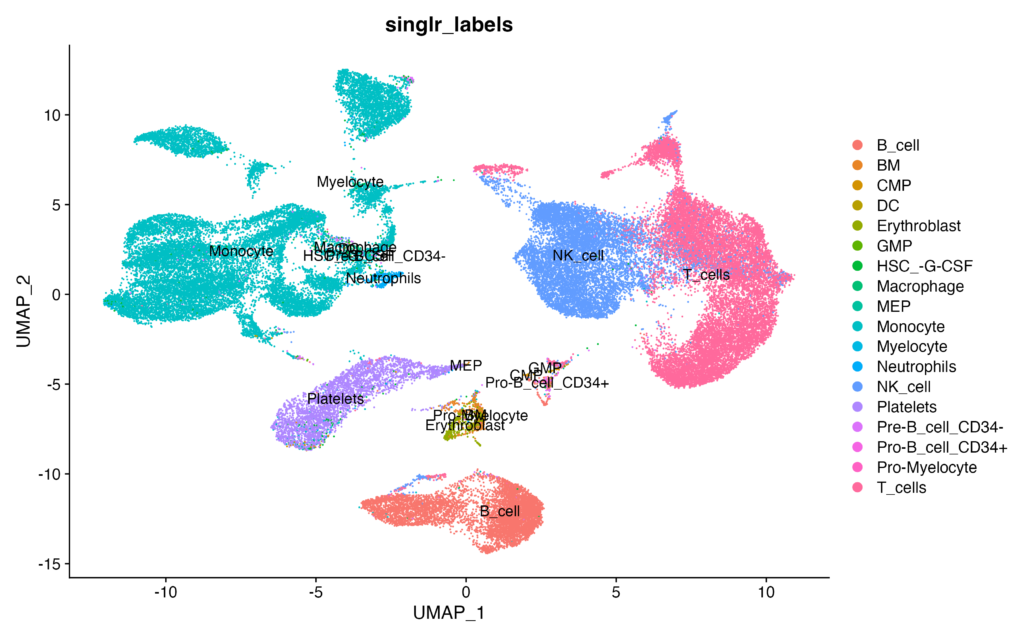
# Visualize cell types in a UMAP plot with labels
DimPlot(pbmc, reduction = 'umap', group.by = 'singlr_labels', label = TRUE)

Execute the code, and if you obtain data similar to the following, it is considered a success:

I will explain the code:

# Check if BiocManager is installed, if not, install it
if (!require("BiocManager", quietly = TRUE))
  install.packages("BiocManager")

# Install required packages using BiocManager
BiocManager::install("SingleR")
BiocManager::install("celldex")
BiocManager::install("SingleCellExperiment")

# Load required libraries
library(SingleR)
library(celldex)
library(SingleCellExperiment)

We are performing library installations.

# Load reference data from celldex
ref <- celldex::HumanPrimaryCellAtlasData()

We use the HumanPrimaryCellAtlasData function from the celldex package to retrieve reference data from the Human Primary Cell Atlas. The reference data is stored in the variable ref.

# Run SingleR to infer cell types of pbmc dataset using reference data
results <- SingleR(test = as.SingleCellExperiment(pbmc), ref = ref, labels = ref$label.main)

We use the SingleR function to estimate the cell types of the pbmc dataset. For this estimation, we use the ref data obtained in the first step as reference data, and we specify ref$label.main as the cell type labels. The estimated cell types are stored in the variable results.

# Add inferred cell type labels to pbmc object
pbmc$singlr_labels <- results$labels

We add the inferred cell type labels from the SingleR estimation to the pbmc object’s metadata, creating a new variable called singlr_labels. This allows us to access and utilize cell type information for visualization and subsequent analyses.

# Visualize cell types in a UMAP plot with labels
DimPlot(pbmc, reduction = 'umap', group.by = 'singlr_labels', label = TRUE)

We create a plot using the DimPlot function, which utilizes UMAP (Uniform Manifold Approximation and Projection) dimension reduction technique. Cells on the plot are grouped based on the cell type labels estimated by SingleR (singlr_labels), and labels are displayed for each group. This visualization allows us to visually inspect the distribution of cell types within the dataset.

FeaturePlot to Confirm Actual Marker Expression

We have successfully assigned each cluster to cell types. However, it’s essential to verify whether the cell types have been correctly assigned. FeaturePlot allows us to visualize the expression of individual genes on the UMAP plot. Let’s use it to check the marker gene expression.

In this case, we will use CD14 as a marker for monocytes and CD3E as a marker for T-cells. Please execute the following:

FeaturePlot(pbmc, features = c("CD14", "CD3E"))

If you obtain the following results, it’s considered successful:

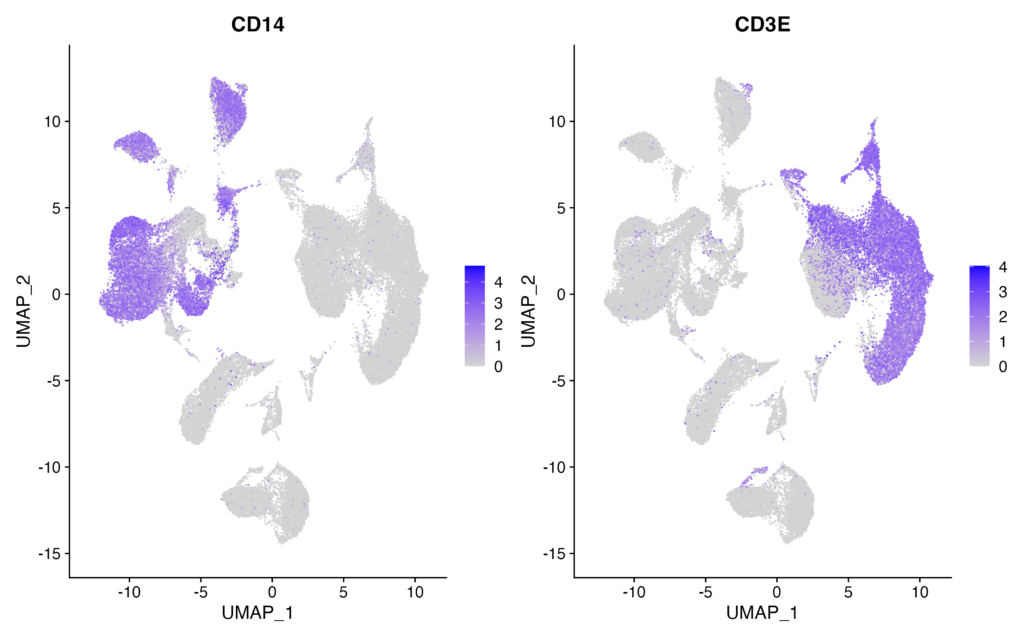
You should see CD14 expression in the clusters assigned as monocytes and CD3E expression in the clusters assigned as T-cells. It’s essential to plot and verify the expression of various marker genes to ensure accurate cell type assignments.

In Conclusion

How was it? While it may not be a complete replication of the figures in the paper, you’ve been able to perform the desired analysis. Please feel free to give it a try!